Wednesday, December 30, 2015

Pascal’s Triangle: Polynomials and TI-84 Plus

Pascal’s Triangle:  Polynomials and TI-84 Plus

Pascal's Triangle

Powers of 2

Pascal’s Triangle holds a great number of properties.   For instance, the sum of each row (R) is a power of two (2^R).  The top row is referred to as row 0.  Hence:

1 = 2^0
1 + 1 = 2 = 2^1
1 + 2 + 1 = 4 = 2^2
1 + 3 + 3 + 1 = 8 = 2^3
1 + 4 + 6 + 4 + 1 = 16 = 2^4
1 + 5 + 10 + 10 + 5 + 1 = 32 = 2^5
1 + 6 + 15 + 20 + 15 + 6 + 1 = 64 = 2^6
and so on…

Binomial Expansion

Take a look what happens when you expand the binomial (x + y)^R:

(x + y)^0 = 1

(x + y)^1 = 1*x + 1*y

(x + y)^2 = 1*x^2 + 2*x*y + 1*y^2

(x + y)^3 = 1*x^3 + 3*x^2*y + 3*x*y^2 + 1*y^3

(x + y)^4 = 1*x^4 + 4*x^3*y + 6*x^2*y^2 + 4*x*y^3 + 1*y^4

(x + y)^5 = 1*x^5 + 5*x^4*y + 10*x^3*y^2 + 10*x^2*y^3 + 5*x*y^4 + 1*y^5

(x + y)^6 = 1*x^6 + 6*x^5*y + 15*x^4*y^2 + 20*x^3*y^3 + 15*x^2*y^4 + 6*x*y^5 + 1*y^6

and so on…

Notice the coefficients (in blue)?  They represent rows of the Pascal’s Triangle. 

Combinatorics

The formula for find the number of combinations of N items from R is:

COMB(R, N) = R nCr N = R! / ((R – N)! * N!)

If you R stand for a row of the Pascal’s Triangle and N stand for an entry (starting from 0), you can get R nCr N from the triangle. 

For instance, for the 4th row (R = 4 with entries 1, 4, 6, 4, 1), 2nd entry (N = 2, with left most entry designated as 0), Pascal’s Triangle will state that 4 nCr 3 = 4! / (2! * 2!) = 6.

For the 5th Row (R = 5):
N = 0, 5 nCr 0 = 1
N = 1, 5 nCr 1 = 5
N = 2, 5 nCr 2 = 10
N = 3, 5 nCr 3 = 10
N = 4, 5 nCr 4 = 5
N = 5, 5 nCr 5 = 1

Sierpinksi Triangle

One of the books I got for Christmas is the book “The Magic of Math: Solving for x and Figuring Out Why” written by Arthur Benjamin.  The book is well written and if you want a good read I recommend this book.  It has something for everyone. One of things I learned from Benjamin’s book is that if you mark all the odd numbers, and you take many rows, you get the famous fractal the Sierpinski Triangle.

Take a look at the diagram below:

Making the Sierpinski Triangle

TI-84 Plus:  Generating a Row of Pascal’s Triangle

A short program to generate a row of Pascal’s Triangle.  The result is stored in list L6.  The first entry is the 0th entry.

Input "ROW:",R
R+1→dim(L₆)
For(K,0,R)
R nCr K→L₆(K+1)
End
Disp "L₆:"
Pause L₆

I think this is self-explanatory.


Eddie

HAPPY NEW YEAR!

Source:

Benjamin, Arthur.  The Magic of Math: Solving for x and Figuring Our Why.  Basic Books:  New York.  2015


This blog is property of Edward Shore.   2015.

Friday, December 18, 2015

Mathematical Art with the HP Prime and TI-84 CE (December 18, 2015 edition)

Mathematical Art with the HP Prime and TI-84 Plus CE (December 18, 2015 edition)

More visuals for your pleasure.  Happy Holidays and Merry Christmas,

Eddie


TI 84 Plus CE: Linear Box Illusion 

HP Prime:  Confetti 2016

HP Prime: The Random-Colored Diamond

HP Prime:  Cutting the Line

HP Prime: A Tear

HP Prime: Open Wide

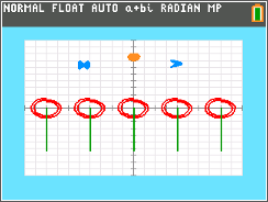
TI-84 Plus CE: Child’s Flowers


This blog is property of Edward Shore. 2015.

Next time will probably be after Christmas!   Thank you all for your support!   Eddie

Sunday, December 13, 2015

Mathematical Art with the HP Prime and TI-84 CE (December 13, 2015 edition)

Mathematical Art with the HP Prime and TI-84 Plus CE (December 13, 2015 edition)

Math is not only fun but can also be creative.  If you want to know I did these plots, please leave a comment below.  Enjoy and best always,

Eddie

HP Prime: Linear Waves

TI -84 Plus CE:  The Arms of Sine

TI-84 Plus CE: Icicles

HP Prime:  Fire From the Flask

TI-84 Plus CE:  Pyramid Illusion

TI-84 Plus CE:  Circular Illusion

HP Prime: Folium Roller Coaster

HP Prime:  Mantra Tiles
This was inspired by this morning's visit to Mantra Coffee in Azusa, CA


The last graphic was inspired by a visit to the Mantra Coffee Company in Azusa, CA (http://www.mantracoffeeco.com/).  


This blog is property of Edward Shore.  2015


Thursday, December 10, 2015

HP Prime and Casio Prizm: 3 Point Neville's Method

HP Prime and Casio Prizm: 3 Point Neville's Method

Introduction

Neville’s Method is an interpolation method to find an approximation of f(x) at point x.  The function may or may not be known.  The method uses Lagrange interpolation polynomials.

For this blog entry, we will work with 3 known points to interpolate a fourth point.  We certainly can use a higher order interpolation if desired or needed.  In general for the 3 known points (x0, y0), (x1, y1), and (x2, y2):

P(0,0)


P(0,1)

P(1,1)

P(0,2)

P(1,2)

P(2,2)


Think of this like a collapsing bracket, collect two neighboring points until a column is completed.  Repeat the process until P(0,n) is reached.   In this case of 3 points, the approximate answer is y ≈ P(0,2).

Formulae:

P(0,0) = (x0, y0)
P(1,1) = (x1, y1)
P(2,2) = (x2, y2)

P(0,1) = ((x1 – x)*y0) + (x – x0)*y1) / (x1 – x0)
P(1,2) = ((x2 – x)*y1) + (x – x1)*y2) / (x2 – x1)

P(0,2) = ((x2 – x)*P(0,1) + (x – x0)*P(1,2)) / (x2 – x0)
Y = P(0,2)

The NEVILLE3 program works with the 3-point interpolation where lists presents the points {x0, x1, x2} and {y0, y1, y2}.  If you use a TI-84 Plus, the Casio Prizm version can be adopted (with appropriate changes).

HP Prime Program:  NEVILLE3

Input:  lx and ly and list of three elements, {x0, x1, x2} and {y0, y1, y2}, respectively, and x is the target point.

EXPORT NEVILLE3(lx,ly,x)
BEGIN
// Neville 3-Point Approx.
// EWS 2015-12-07

LOCAL la,a,y,k,n;

la:={0}; // for consistency

FOR k FROM 1 TO 3 DO

IF k==3 THEN
a:=((lx(3)-x)*la(2)+(x-lx(1))*
la(3))/(lx(3)-lx(1));
ELSE

a:=((lx(k+1)-x)*ly(k)+(x-lx(k))*
ly(k+1))/(lx(k+1)-lx(k));
END;
la:=CONCAT(la,{a});
END;
y:=la(4); RETURN y;
END;


Casio Prizm Program NEVILLE3

Input:  List 1 and List 2 and list of three elements, {x0, x1, x2} and {y0, y1, y2}, respectively, and x is the target point.

“3 PT NEVILLE”
“LIST X”? → List 1
“LIST Y”? → List 2
“X?” → X
{0} → List 3
For 1 → K To 3
If K = 3
Then
(( List 1[3] – X ) * List 3[2] + ( X – List 1[1]) * List 3[3] )
÷ (List 1[3] – List 1[1]) → A
Else
(( List 1[K+1] – X ) * List 2[K] + (X – List 1[K]) * List 2[K+1] )
÷ (List 1[K+1] – List 1[K] ) → A
IfEnd
Augment(List 3,{A}) → List 3
Next
List 3[4] → Y
Y


Examples:

Example 1;
List X/List 1 = {16, 64, 100}
List Y/List 2 = {0.25, 0.125, 0.1}
X = 81

Result:  0.1058511078

Example 2:
List X/List 1 = {-2, 0, 2}
List Y/List 2 = {11, 4, 11}
X = 3

Result:  19.75


Sources:

Mitchell, Kevin.  “Neville’s Method”  Simon Fraser University. MACM 316 – Fall 2010.   http://people.math.sfu.ca/~kevmitch/teaching/316-10.09/neville.pdf    Retrieved December 4, 2015

Wikiversity.  “Topic:  Numerical analysis/Neville’s algorithm examples”  https://en.wikiversity.org/wiki/Topic:Numerical_analysis/Neville%27s_algorithm_examples  Retrieved December 4, 2015


This blog is property of Edward Shore.  2015

Friday, December 4, 2015

HP Prime: Slopefield (Differential Equations)

HP Prime:  Slopefield (Differential Equations)

Here is a program that graphs the slopefield of a differential equation in the form dy/dx = f(x,y).  This program is adopted from Alan Ziv’s SLPFIELD program, which Ziv programmed for the Casio fx-9850G.  The link to the original program is here:  http://www.spiderpixel.co.uk/caspro/progs/9x50g/slopefield.txt


For the HP Prime version, enter dy/dx in quotes, and use capital letters X and Y.  I recommend that you are in the Function app for this.  The window should be set up before running SLOPEFIELD.

Program SLOPEFIELD

EXPORT SLOPEFIELD(dxy)
BEGIN
// dxy: dx/dy = f′(x,y)
// Adopted from Alan Ziv -
// Casio
// dxy is in quotes
LOCAL X,Y,C,D,J,K,G,H;
LOCAL F,xa,xb,ya,yb,E;

// Use the Function App
RECT();
C:=(Ymax-Ymin)/220;
D:=(Xmax-Xmin)/320;

FOR J FROM 0 TO 50 DO
E:=Xmin+(8*J+3)*D;
FOR K FROM 0 TO 27 DO
F:=Ymin+(8*K+3)*C;

X:=E;
Y:=F;
G:=EXPR(dxy);
H:=2*D;

IF ABS(G)>C/D THEN
H:=2*C/ABS(G);
END;

IF 2*H>D THEN
xa:=E-H; ya:=G*(xa-E)+F;
xb:=E+H; yb:=G*(xb-E)+F;
LINE(xa,ya,xb,yb);
ELSE
LINE(E,F+2*C,E,F-2*C);
END;
END;
END;

// Draw Axis
LINE(Xmin,0,Xmax,0,#C0C0C0h);
LINE(0,Ymin,0,Ymax,#C0C0C0h);
WAIT(0);

END;

 Examples:

dy/dx = X*^Y^2 + 3*X

 
dy/dx = Y*SIN(X)

This blog is property of Edward Shore.  2015

Eddie


HP Prime: Gauss-Jordan Elimination Method

HP Prime:  Gauss-Jordan Elimination Method

I received an email requesting some programs of various numerical methods.   One of the methods is the Gauss-Jordan Elimination Method. 

Basically, the Gauss-Jordan Elimination Method is a step-by-step method of matrix row operations to reduce a matrix A = [ X | Y ] where X is (mostly) a square component joined by a column vector Y to the form [ I | R ], which I represents an identity matrix portion where the diagonal elements are 1. 

You can quickly execute the method by use of the RREF (Reduced Row Echelon Form) function, which is present on many graphing calculators (if not all of them these days). 

The HP Prime program GAUSSJORDAN is shows a step by step method.  What the program does is:

1. Take the dimensions of the matrix.
2. Starting with column 1, pivot on element (1,1).  This is accomplished by one of two operations.  SCALEADD which multiplies the first row by a factor and adds it to a target row k.  The goal is reduce the element (k,1) to 0, for all k ≠ 1.
3. Once step 2 is completed, the SCALE command is used to divide the value of element (1,1) to reduce it to 1, if necessary.
4. Repeat steps 2 and 3 for each column until the number the rows is reached.

Notes:

1. HP Prime’s SCALEADD is the *Row+ command for the Casio and TI graphing calculators.  Similarly, HP Prime’s SCALE is the *Row command for the Casio and TI graphing calculators. 
2. The program requires that the matrix have all elements that are (1,1), (2,2), (3,3), etc. are non-zero.  Otherwise an error occurs.  You can swap rows by the rowSwap command if necessary to get the matrix in proper form.
3. While the program GAUSSJORDAN shows you step by step, it shows one order of approach, which may or may not be the most efficient number of steps.
4.  If the HP Prime is in Standard mode, you may see 0.9999999999999 or some number to the 10^-13 power.   This is due to the rounding mechanisms.  Feel free to round these numbers to 1 and 0, respectively.

With all this in mind, here is the program: 

Program GAUSSJORDAN

EXPORT GAUSSJORDAN(mat)
BEGIN
// Guass-Jordan Elimination
// 2015-12-04
// Matrix MUST have
// mat[k,k]≠0

LOCAL l,r,c,j,k,h,v;
PRINT();

l:=SIZE(mat);
r:=l[1]; c:=l[2];
j:=1;

// Main row loop
FOR k FROM 1 TO r DO

// Secondary row loop
FOR h FROM 1 TO r DO

// k = target row
// h = test row
// Pivot operation
IF h≠k THEN
v:=−mat[h,k]/mat[k,k];
mat:=SCALEADD(mat,v,k,h);
PRINT();
PRINT("After Step "+j);
PRINT(mat);
WAIT(0);
j:=j+1;
END;

IF mat[k,k]≠1 THEN
v:=1/mat[k,k];
mat:=SCALE(mat,v,k);
PRINT();
PRINT("After Step "+j);
PRINT(mat);
WAIT(0);
j:=j+1;
END;

END;
END;

PRINT();
PRINT("Result:");
PRINT(mat);

// Final WAIT not needed

RETURN mat;

END;


Examples:

M2 = [[1,2,4,1] [3, -3, 3, 0] [6, 6, 8, 5]]
Final Result* (see Note 4) of GAUSSJORDAN(M2):
[[1,0,0,0.53333333333]. [0,1,0,0.43333333333], [0,0,1,-0.1]]

M3 = [[0,4,-1,-1], [2,5,2,2], [3,3,6,3]].
Running GAUSSJORDAN(M3) with M3 as is will get an error.  Why?  See M3[1,1] = 0.  We must make it non-zero.  Do this by swapping rows.
M3≔rowSwap(M3,1,2) to make the matrix [[2,5,2,2], [0,4,-1,-1], [3,3,6,3]].  Now you are ready to go.
GAUSSJORDAN(M3) returns [[1,0,0,2.6], [0,1,0,-0.4], [0,0,1,-0.6]]

Thank you Luis for the email and the suggestions. 


Source:  Cazelais, Gilles. “Gauss-Jordan Elimination Method”  http://pages.pacificcoast.net/~cazelais/251/gauss-jordan.pdf  Retrieved December 4, 2015


Until next time, stay safe everyone because it is a crazy planet we live on. 


Eddie