Sunday, March 26, 2023

HP 32S II Statistical Formulas

HP 32S II Statistical Formulas


Statistics Formulas


The 32S II can store formulas for evaluations, including formulas involving stat variables.  


Covariance:

C = r × sx × sy


Root Mean Square Based on X Variable Statistics:

R = SQRT( Σx^2 ÷ n )


Z-Score Based on X Variable Statistics:  

Z = (X - x-bar) ÷ sx


Accessing Stat variables:


r:  [ right shift ]  [ LN ] (L.R.) [ y^x ] (r)

sx:  [ right shift ] [ 1/x ] (s, σ), [ √x ] (sx)

sy:  [ right shift ] [ 1/x ] (s, σ), [ LN ] (sy)

Σx^2:  [ right shift ] [ Σ+ ] (SUMS) [ e^x ] (x)

n:  [ right shift ] [ Σ+ ] (SUMS) [ √x ] (n)

x-bar:  [ right shift ] [ y^x ] (x-bar,y-bar) [ √x ] (x-bar)


Example


Data:  (x, y)

(10.4, 20)

(13.5, 18)

(16.8, 15)

(19.1, 13.9)


Enter statistical data:  y [ENTER] x [ Σ+ ]


Some stats:

x-bar = 14.95

y-bar = 16.725

r = -9.9503133E-1


Covariance:  Solve for C

C = -10.555

Result is stored in C


Root Mean Square:  Solve for R

R = 15.3089842903

Result is stored in R


Z-Score Based on X Variable Statistics:   Solve for Z

X?  15,  Z = 1.31382E-2

X?  17,  Z = 5.38666E-1

Result is stored in Z


Formulas vs. Programs


If we are going to evaluate formulas (that is, solve for the variable left of the equals sign), we could also enter and use programs.   The programs for the above three formulas:


Covariance:

C01  LBL C

C02  r

C03  sx

C04  ×

C05  sy

C06  ×

C07  RTN


Root Mean Square:

R01  LBL R

R02  Σx^2

R03  n

R04  ÷

R05  SQRT

R06  RTN


Z Score:  (x is in the X stack)

Z01  LBL Z

Z02  x-bar

Z03  -

Z04  sx

Z05  ÷

Z06  RTN


Byte Consumption Comparison


Covariance

Formula:  12 bytes

Program:  10.5 bytes


Root Mean Square

Formula:  12 bytes

Program:  9 bytes


Z Score

Formula: 15 bytes

Program:  9 bytes


From sample set, programs are shorter than formulas.  Is this true in general?


Eddie


All original content copyright, © 2011-2023.  Edward Shore.   Unauthorized use and/or unauthorized distribution for commercial purposes without express and written permission from the author is strictly prohibited.  This blog entry may be distributed for noncommercial purposes, provided that full credit is given to the author. 


Saturday, March 25, 2023

HP 10bII+ and Sharp EL-W516T: Normal Distribution Function

HP 10bII+ and Sharp EL-W516T:  Normal Distribution Function


Sometimes scientific calculators and financial calculators have normal distribution functions.   


HP 10bII+  Normal Distribution


On the HP 10bII+ financial calculator, the normal distribution functions are available at any time:


[ blue shift ] ( z<>p ):   lower tail area of normal distribution [ P(x) ]

[ blue shift ] ( INV) ( z<>p ):  given area, get the probability


Example:


P(0.2) returns 0.57926


If the area is 0.6, z is 0.253347


Sharp EL-W516T Normal Distribution


The normal distribution functions offered on the Sharp EL-W516T are:


[ MATH ] menu in SD mode:

0) →t:   convert to z

1)  P(:  lower tail area

2)  Q(:  I do believe it is the area between the mean and z

3)  R(:  upper tail area


The normal distribution functions are available only in the statistics mode.  


Example:


P(0.2) returns 0.57296.


Is Statistical Data Required?


No.  In general, especially the normal distribution functions does not require or depend on any stat data.  


However, you use the stat data points to convert from x-values to convert stats to a z value in the EL-W516T using →t.  Here is an example:


Data set:  -3, -1, 2, 5, 6 

Convert the data point 0 and then find the lower tail area.


0→t=   -0.524890659

P(ANS) = 0.29983


Eddie


All original content copyright, © 2011-2023.  Edward Shore.   Unauthorized use and/or unauthorized distribution for commercial purposes without express and written permission from the author is strictly prohibited.  This blog entry may be distributed for noncommercial purposes, provided that full credit is given to the author. 


Sunday, March 19, 2023

HP 12C: An Improved Linear Regression Function (from Curvee RPN-45 SD)

HP 12C:  An Improved Linear Regression Function (from Curvee RPN-45 SD)


Curvee RPN-45 Simulator 


The Curvee RPN-45 from Curvee Software is an excellent app.  The RPN-45 SD app is the Super-45.   The Super-45 is a emulator of the classic HP 45 calculator from 1973 with the following enhancements:


*  The gold shift key becomes a double-shift key (gold/purple)

*  Complex Numbers

*  10 additional registers

*  Days between dates

*  Four solvers: 2 x 2 system of linear equations, 3 x 3 system of linear equations, quadratic equation, cubic equation

*  Expanded statistics including full linear regression analysis


I have purchased one on my iPod Touch (that is an iPhone without the "phone" part) for $1.99 (prices may vary).  There are versions for the iPhone and iPad.  


For more information:  http://cuveesoft.ch/rpn45/en/index.html


The enhanced linear regression (L.R.) function on the Super-45 returns the following calculations to the four-level stack:


T:  covariance

Z:  correlation

Y:  slope

X:  intercept


The relationship between correlation (r) and covariance (cov):


cov(x,y) = r * sx * sy

sx = standard deviation of x-data

sy = standard deviation of y-data


The HP 12C mimics the enhanced L.R. function.   Yes, check out this app!


HP 12C Program:  Enhanced Linear Regression


The results are stored in the following registers:


R7 = intercept

R8 = Slope

R9 = correlation

R.0 = covariance


In addition, I added code to calculate population deviation:  σx in the x-stack, σy in the y-stack.


Step #: Code [ key ]


// linear regression function 

01:  1  [ 1 ]

02:  43, 1  [ x^,r ]

03:  34  [ x<>y ]

04:  44, 9 [ STO 9 ]

05:  43, 48  [ s ]

06:  20  [ × ]

07:  20  [ × ]

08:  44, 48, 0   [ STO  .  0  (decimal point, zero) ]

09:  0  [ 0 ]

10:  43, 2  [ y^, r ]

11:  44, 7  [ STO 7 ]

12:  1   [  1 ]

13:  43, 2  [ y^, r ]

14:  34  [ x<>y ]

15:  33  [ R↓ ]

16:  34  [ x<>y ]

17:  30  [ - ]

18:  44, 8 [ STO 8 ]

19:  45, 48, 0 [  RCL . 0  (decimal point, zero) ]

20:  45, 9  [ RCL 9 ]

21:  45, 8  [ RCL 8 ]

22:  45, 7  [ RCL 7 ]

23:  43, 33, 00 [ GTO 00 ]


// population deviation

24:  45, 1 [ RCL 1 ]

25:  36  [ ENTER ]

26:  36  [ ENTER ]

27:  1  [ 1 ]

28:  30  [ - ]

29:  10  [ ÷ ]

30:  43, 21  [ √ ]

31:  44, 0  [ STO 0 ]

32:  43, 48  [ s ]

33:  45, 0  [ RCL 0 ]

34:  10  [ ÷ ]

35:  34  [ x<>y ]

36:  45, 0  [ RCL 0 ]

37:  10  [ ÷ ]

38:  34  [ x<>y ]

39:  43, 33, 00 [ GTO 00 ]


Example


Fix 6 mode is set.  


Data:

(5.35, 10)

(5,70, 11)

(6.18, 12)

(6.55, 13)

(6.97, 14)

(7.36, 15)


After entering the data points:

[ f ] (PRGM) [ R/S ]

-3.162788 (intercept), [ R↓ ]

2.465287 (slope), [ R↓ ]

0.999396 (correlation, r), [ R↓ ]

1.418000 (covariance)  ( [ R↓ ] to return the stack to it's original configuration )


[ g ] (GTO) 24 [ R/S ]

0.692331 ( σx ) [ x<>y ]

1.707825 ( σy )


Eddie


All original content copyright, © 2011-2023.  Edward Shore.   Unauthorized use and/or unauthorized distribution for commercial purposes without express and written permission from the author is strictly prohibited.  This blog entry may be distributed for noncommercial purposes, provided that full credit is given to the author. 


Saturday, March 18, 2023

TI-84 Plus CE: Tracing Polar Equations

TI-84 Plus CE:  Tracing Polar Equations


Traveling Around the Graphs


The programing BLINKING animates a dot around one of four polar equations:


1.  Ellipse


r = b / √(1 - ε^2 * cos^2 θ), where ε = √(a^2 - b^2)/a, a > b


2.  Cardioid


r = a + (1 + cos θ)


3.  3-Leaf Rose


r = a * cos(3 * θ)


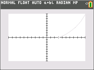
4.  Log Spiral


r = a * e^(b * θ)


Notes:


The point alternates through blue (TI-84 Plus CE color 10), green (14), orange (15), and black (12).   The graph itself is light gray (21).  


r1 is the polar equation r1(θ).


Plotting points (not the polar graph) must be in cartesian coordinates (x,y).   


TI-84 Plus CE Program:  BLINKING


"2023-01-15 EWS"

Radian: Polar: FnOff

ZStandard

{10,14,15,12}→L6

Menu("PLOT","ELLIPSE",10,"CARDIOID",11,"3-LEAF ROSE",12,"LOG SPIRAL",13)


Lbl 10

Disp "A≥B"

Prompt A, B

√(A^2-B^2)/A→E

"B/√(1-E^2*cos(θ)^2)"→r1

Goto 20


Lbl 11

Prompt A

"A*(1+cos(θ))"→r1

Goto 20


Lbl 12

Prompt A

"A*cos(3*θ)"→r1

Goto 20


Lbl 13

Disp "A>0, B>0"

Prompt A,B

"A*e^(B*θ)"→r1

Goto 20


Lbl 20

Input "MAX? ",M

Input "NO. STEPS? ",S

M/S→N

FnOn 1

GraphColor(1,21)

0→P: r1(P)→Q

P>Rx(Q,P)→F: P>Ry(Q,P)→G

Pt-On(F,G,1,12)


For(K,1,S)

Wait 0.25

Pt-On(F,G,1,21)

remainder(K,4)+1→C

K*N→P: r1(P)→Q

P>Rx(Q,P)→F: P>Ry(Q,P)→G

Pt-On(F,G,1,L6(C))

End 


Disp "END"


Examples


In all examples, a = 3, b = 2, maximum = 4 * π, steps = 24


Ellipse


Cardioid


3-Leaf Rose


Log Spiral


Source


Harris, John W. and Horst Stocker.  Handbook of Mathematics and Computational Science  Springer:  New York.  2006.  ISBN 0-387-94746-9


Eddie


All original content copyright, © 2011-2023.  Edward Shore.   Unauthorized use and/or unauthorized distribution for commercial purposes without express and written permission from the author is strictly prohibited.  This blog entry may be distributed for noncommercial purposes, provided that full credit is given to the author. 


Thursday, March 16, 2023

Python - Pride and Transgender Flag

Python - Pride and Transgender Flag


The fact that we don't have equality and there are elected officials whose agenda is to destroy civil rights on this planet is ridiculous.  Enough is enough. 


I stand with the LGTBQ community.  Now and forever.   - EWS


Python Code Using Casio MicroPython


Download here:  https://drive.google.com/file/d/1ZSGR_ayEOIwbjsEiNtINCmIhbs7yo0zt/view?usp=share_link


Pride Flag:  pride50.py


# pride flag


from casioplot import *


clear_screen()


for i in range(5,376):

  for k in range(5,35):

    set_pixel(i,k,(228,3,3))


for i in range(5,376):

  for k in range(35,65):

    set_pixel(i,k,(255,140,0))


for i in range(5,376):

  for k in range(65,95):

    set_pixel(i,k,(255,237,0))


for i in range(5,376):

  for k in range(95,125):

    set_pixel(i,k,(0,128,38))


for i in range(5,376):

  for k in range(125,155):

    set_pixel(i,k,(36,64,142))


for i in range(5,376):

  for k in range(155,185):

    set_pixel(i,k,(115,41,130))


show_screen()    


Transgender Flag:  trans50.py


# transgender flag


from casioplot import *


clear_screen()


for i in range(5,376):

  for k in range(5,41):

    set_pixel(i,k,(91,206,250))


for i in range(5,376):

  for k in range(41,77):

    set_pixel(i,k,(245,169,184))


for i in range(5,376):

  for k in range(77,113):

    set_pixel(i,k,(255,255,255))


for i in range(5,376):

  for k in range(113,149):

    set_pixel(i,k,(245,169,184))


for i in range(5,376):

  for k in range(149,185):

    set_pixel(i,k,(91,206,250))


show_screen()    


Python Code Using the Turtle Module from Numworks


Download here:  https://drive.google.com/file/d/1odztGLGfyRsVwq5xSBrfIrc27pj7v58i/view?usp=share_link


Pride Flag:  pride50.nw


from math import *

from turtle import *


hideturtle()

speed(10)


# have to keep size to 1

# want box quality


color(228,3,3)

for i in range(90,60,-1):

  penup()

  goto(-140,i)

  pendown()

  forward(280)


color(255,140,0)

for i in range(60,30,-1):

  penup()

  goto(-140,i)

  pendown()

  forward(280)


color(255,237,0)

for i in range(30,0,-1):

  penup()

  goto(-140,i)

  pendown()

  forward(280)


color(0,128,38)

for i in range(0,-30,-1):

  penup()

  goto(-140,i)

  pendown()

  forward(280)


color(36,64,142)

for i in range(-30,-60,-1):

  penup()

  goto(-140,i)

  pendown()

  forward(280)


color(115,41,130)

for i in range(-60,-90,-1):

  penup()

  goto(-140,i)

  pendown()

  forward(280)


Transgender Flag:  transnw.py


from math import *

from turtle import *


hideturtle()

speed(10)


# have to keep size to 1

# want box quality


color(91,206,250)

for i in range(90,54,-1):

  penup()

  goto(-140,i)

  pendown()

  forward(280)


color(245,169,184)

for i in range(54,18,-1):

  penup()

  goto(-140,i)

  pendown()

  forward(280)


color(255,255,255)

for i in range(18,-18,-1):

  penup()

  goto(-140,i)

  pendown()

  forward(280)


color(245,169,184)

for i in range(-18,-54,-1):

  penup()

  goto(-140,i)

  pendown()

  forward(280)


color(91,206,250)

for i in range(-54,-90,-1):

  penup()

  goto(-140,i)

  pendown()

  forward(280)


color(91,206,250)

for i in range(90,54,-1):

  penup()

  goto(-140,i)

  pendown()

  forward(280)


Source:


"Pride (Rainbow) Flag Color Codes"  flagcolorcodes Retrieved March 15, 2023.

https://www.flagcolorcodes.com/pride-rainbow


"Transgender Flag Color Codes"   flagcolorcodes.  Retrieved March 15, 2023. 

https://www.flagcolorcodes.com/transgender


Eddie 


All original content copyright, © 2011-2023.  Edward Shore.   Unauthorized use and/or unauthorized distribution for commercial purposes without express and written permission from the author is strictly prohibited.  This blog entry may be distributed for noncommercial purposes, provided that full credit is given to the author. 

Tuesday, March 14, 2023

Casio Classpad (fx-CP400): Collection of Functions

Casio Classpad  (fx-CP400):  Collection of Functions


For my birthday post, on Pi (π) Day (March 14), here is a collection of functions for the Casio Classpad (300, 330, fx-CP400, fx-CP500). 


Birthday Probability Function:   bday(c,n)


"The probability that a number in a room do not share a same birthday"

c:  number of categories (i.e. days in a year)

n:  population size


Example:

bday(365, 40):  0.1087681902


Percent Change:  pchg(old, new)


old:  old amount

new:  new amount


Example:

pchg(400,500):  25


Combination with Repetition:  nHr(n,r)


n:  population

r:  number of objects to pick


Example:

nHr(52,5):  3819816


Error Function and Error Compliment Function


Error Function:   erf(x)

Error Compliment Function:  erfc(x)


Note that erf(x) + erfc(x) = 1


Example:

erf(0.60):  0.6038560908

erfc(0.60):  0.3961439092


Law of Cosines


a^2 = b^2 + c^2 - 2*b*c*cos(α)


Finding the Angle α:  cosang(a,b,c)

Finding the Side a:  cosside(b,c,α)


Example:

(Degrees Mode)

a = 20.1, b = 18.5, c = 22.3:  cosang(20.1,18.5,22.3):  58.13961834°  (approx)

b = 24.2, c = 18.9, α = 58°:  cosside(24.2,18.9,58):  21.4032954 (approx)


Fresnel Integrals


Fresnel Cosine Integral:  frescos(u)

C(u) = ∫( cos(π * x^2 ÷ 2) dx, 0, u)


Fresnel Sine Integral:  fressin(u)

S(u) = ∫( sin(π * x^2 ÷ 2) dx, 0, u)


Example:

frescos(1.5):  0.445261176

fressin(1.5):  0.6975049601


Bessel Integral of the First Kind:  bessel(n,x)


J_n(x) = 1 / π * ∫( cos(n * t - x * sin t) dt, 0, π)


Example:

bessel(0,1.5):  0.5118276716

bessel(2,1.2):  0.1593490183


Elliptic Integral of the First Kind:  ellip(x)


K(x) = ∫( 1/ √(1 - x^2 * sin^2 t) dt, 0, π/2)


Example:

ellip(-0.6):  1.750753803

ellip(0.4):  1.639999866


Sine Integral:  Si(x)


Si(x) = ∫( sin t / t dt, 0, x)


Example:

Si(1.8):  1.50581678

Si(6):  1.424687551


Beta Function:  beta(a,b)


β(a, b) = (Γ(a) * Γ(b)) ÷ Γ(a+b)


Example:

beta(2,3): 1/12

beta(1.9,4.6):  0.04470413922 (approx)


Relativity Factor:  relat(v)


factor = √(1 - v^2/c^2)

c = 299792458 m/s

v = velocity


Example:

relat(201E6):  0.7419422153  (approx)


Schwarzschild Radius:  schwarz(m)


r = (2 * G * m)/c^2

G = 6.674E-11  m^3/(kg s^2)

c = 299792458 m/s

m = mass the black hole, kg

r = Schwarzschild Radius, m  (event horizon)


Example:

schwarz(7.89E30):  11717.95418


Distance of a Drop:  dropdist(v0,t)


v0:  initial velocity, m/s

t: time, s

Calculated:  distance, m


Example:

dropdist(15,5):  197.583125


Cycle of a Simple Pendulum:  pendu(l)


l:  length of a string, m

Calulated:  time of the pendulum swing, s


Example:  

pendu(5.5):  4.705446883


Impedance in LRC Series Circuit:  lrcser(R,f,L,C)


R:  resistance, Ω

f:  frequency, Hz

L:  inductance, H

C:  capacity, F


Example:

lrcser(4,80,0.1,50E-6):  11.21437564


Impedance in LRC Parallel Circuit:  lrcpar(R,f,L,C)


R:  resistance, Ω

f:  frequency, Hz

L:  inductance, H

C:  capacity, F


Example:

lrcpar(4,80,0.1,50E-6):  3.999122191


Source for:

Distance of a Drop

Cycle of a Simple Pendulum

Impedance in LRC Series Circuit

Impedance in LRC Parallel Circuit


Scientific Calculator 128 fx-1000F/fx-5000F Owner's Manual.   Casio.  Tokyo, Japan. 


Download the file here:  https://drive.google.com/file/d/1M54HlJ9dP95VBEmGzkUozGzJxKGpiHMh/view?usp=share_link


Eddie 


All original content copyright, © 2011-2023.  Edward Shore.   Unauthorized use and/or unauthorized distribution for commercial purposes without express and written permission from the author is strictly prohibited.  This blog entry may be distributed for noncommercial purposes, provided that full credit is given to the author. 


Monday, March 13, 2023

Review: TI-83 Premium CE Python Edition

Review: TI-83 Premium CE Python Edition


Quick Facts


Model: TI-83 Premium CE Python Edition

Company: Texas Instruments

Price:  $90 - $130 US Dollars 

Country of Origin:  France

Power:  Rechargeable

USB Cord:  Standard A to Mini-B

Memory:  154,000 bytes RAM, 3MB ROM

Display size:  color, backlit, 240 x 320 pixels

Operating System:  Algebraic

Are programs compatible with TI-84 Plus CE?  Yes, both TI-BASIC and Python programs through TI Connect CE.

Essentially the TI-83 Premium CE Python Edition and TI-84 Plus CE Python (of the United States) are similar.   The French TI-83 Premium CE Python was first released in 2019, two years prior to the TI-84 Plus CE Python.   

I note at this time, March 2023, finding TI-84 Plus CE Python calculators to buy are extremely hard to find due to global chip shortage.   

The TI-83 Premium CE Python Edition is based off of the TI-83 Premium CE but it has an additional ARM chip that gives the calculator the Python, specifically CircuitPython.  We have a similar structure for the TI-84 Plus CE Python.  

My review on the American TI-84 Plus CE Python:  http://edspi31415.blogspot.com/2021/07/review-ti-84-plus-ce-python.html

The rest of the blog is going to highlight some comparisons and unique features.


QPiRac:  The Exact Calculator Engine


I wish the TI-84 Plus CE had this:  exact calculations, which is known as QPiRac.  


Q:  fractions

Pi:  terms of π

Rac:  radicals (square roots)


The TI-36X Pro (and TI-30X Pro MathPrint) also has exact math.   We can convert between approximate and exact answers by pressing the [ <> ] button.  


Keyboard Differences


TI-83 Premium CE Python keypad:


TI-84 Plus CE Python keypad:


A lot of the keys between the TI-83 Premium CE and the TI-84 Plus CE (and their respective Python editions) differ even though the features between the two calculators are pretty much the same.  Keep in mind the keys on the TI-83 Premium CE are in French, while the keys on the TI-84 Plus CE are in English.  


*  The fraction shortcut template is a shortcut is accessed on the TI-84 Plus CE by the key sequence  [ alpha ] [ X,T,θ,n ].   On the TI-83 Premium CE, the fraction template is its own key.


*  The reciprocal function is a primary key on the TI-84 Plus CE, but it is a secondary function of the matrix key, [ matrice ], on the TI-83 Premium CE.


*  Speaking of matrices, the menu is a primary key on the TI-83 Premium CE, mainly the [ matrice ] key.  


*  Instead of separate keys, all the trigonometric and inverse trigonometric functions are accessed by the [ trig ] key on the TI-83 Premium CE.  


*  The solver and the PlySmlt2 (polynomial and simultaneous equations) are accessed by the [ résol ] key on the TI-83 Premium CE.


*  The TI-83 Premium CE has a template popup menu, accessed by pressing [ 2nd ] [ []/[] ] (∫ [] d []>).


*  The [ annul ] key on the TI-83 Premium CE is the [ clear ] key on the TI-84 Plus CE.


*  The [ suppr ] key on the TI-83 Premium CE is the [ del ] (delete) key on the TI-84 Plus CE.


*  The insérer function on the TI-83 Premium CE is the ins (insert) function on the TI-84 Plus CE.


*  The applications key is moved to the 2nd function on the [ résol ] key.  


*  The pi (π) constant is a 2nd function of the [ ^ ] key on the TI-84 Plus CE, but the 2nd function of the [ trig ] key on the TI-83 Premium CE.  


*  The stats menu on the TI-83 Premium CE has a Quartiles Setting, something that is not present on the TI-84 Plus CE.   I did not realize that there are different methods to determine quartiles.   The options presented are TI-83CE method and TI-8x method.  This is something I have to read about.  


Final Thoughts


I like the TI-83 Premium CE Python Edition, it's got the exact math engine, and it's not just limited to the Home Screen.  The exact math engine extends to the all the apps except for Python.  Even TI-Basics programs have the exact math engine, which is a pleasant surprise.   If you are looking for a TI Python but not an Nspire, the TI-83 Premium CE Python Edition is worth checking out.  

Still hoping for more color options and the base conversions.


Sources


Shore, Edward.   "Review: TI-84 Plus CE Python"  Eddie's Math and Calculator Blog.  July 19, 2021.  http://edspi31415.blogspot.com/2021/07/review-ti-84-plus-ce-python.html


"TI-83 Premium CE"  Wikipedia.  Last Updated October 25, 2021.  Accessed March 2, 2023.  https://en.wikipedia.org/wiki/TI-83_Premium_CE


Woerner, Joerg.  "TI-83 Premium CE Edition Python"  Datamath Calculator Museum.   May 30, 2019.  http://www.datamath.org/Graphing/TI-83PRCE.htm


Eddie


All original content copyright, © 2011-2023.  Edward Shore.   Unauthorized use and/or unauthorized distribution for commercial purposes without express and written permission from the author is strictly prohibited.  This blog entry may be distributed for noncommercial purposes, provided that full credit is given to the author. 


Sunday, March 12, 2023

Casio fx-CG50: Logistic Equation - Solving For Parameters From Two Data Points

Casio fx-CG50:  Logistic Equation - Solving For Parameters From Two Data Points


The Challenge


It can be a challenge, especially without a statistics software package or method like the maximum likelihood estimate, to fit data (x, p), to the curve:


p(x) = 1 / ( 1 + α * x^β ) = ( 1 + α * x^β )^-1


What happens if we just have two data points (x1, p1) and (x2, p2).  Then finding α and β turns into simpler task.   Either we find a quick estimate to extend to other data points or if we just have two data points, exact solutions.


Finding α and β


With the points (x1, p1) and (x2, p2), the system to solve is:


1 / ( 1 + α * x1^β ) = p1

1 / ( 1 + α * x2^β ) = p2


1 + α * x1^β = 1/p1

1 + α * x2^β = 1/p2


α * x1^β = 1/p1 - 1

α * x2^β = 1/p2 - 1 


Assuming that α ≠ 0, divide both equations to get:


x1^β / x2^β = (1/p1 - 1) / (1/p2 - 1)


Solve for β:


(x1/x2)^β = (1/p1 - 1) / (1/p2 - 1)


ln [ (x1/x2)^β  ] = ln [ (1/p1 - 1) / (1/p2 - 1) ]


β * ln [ (x1/x2) ] = ln [ (1/p1 - 1) / (1/p2 - 1) ]


β = ln [ (1/p1 - 1) / (1/p2 - 1) ] / ln [ (x1/x2) ] 


Then we can get α:  


α = (1/p1 - 1) / (x1^β) = (1/p2 - 1) / (x2^β) 


Casio fx-CG50 Program:  BETPARAM

(276 bytes)


The characters α and β are found in the CHAR sub menu (outside of the PRGM menu).  If you have a monochrome calculator or just don't want color, ignore the color commands.


The program then graphs the resulting equation.   The variables Y1 and Y2 (with the bold Y) represent functions of X.  


Red "P(X)=1÷(1+αX^β)"

"SOLVE FOR α, β"◢

Rad

"POINT 1"

"X1"?→Y

"P1"?→Q

"POINT 2"

"X2"?→Z

"Y2"?→R

ln ((Q^-1 -1)÷(R^1 - 1))

Ans÷ln (Y÷Z)→B

(Q^-1 - 1)÷(Y^B)→A

ClrText

Blue Locate 1,3,"EST. PARAMETERS"

Locate 1,4,"α="

Locate 5,4,A

Locate 1,5,"β="

Locate 5,5,B

"1÷(1+A×X^B)"→Y1

""→Y2

SetG-Color Green,1

DrawGraph

ZoomAuto


Examples


Example 1:

(x1, p1) = (0.5, 0.76)

(x2, p2) = (1.5, 0.70)


Example 2:

(x1, p1) = (3/2, 5/8)

(x2, p2) = (2/3, 3/8)


Source:


Sumpter, David.  The Ten Equations That Rule the World: And How You Can use Them Too.  Flatiron Books: New York.  2021.  ISBN 978-1-250-24696-7


Eddie


All original content copyright, © 2011-2023.  Edward Shore.   Unauthorized use and/or unauthorized distribution for commercial purposes without express and written permission from the author is strictly prohibited.  This blog entry may be distributed for noncommercial purposes, provided that full credit is given to the author.