HP Prime: Custom Menu Using a User Key

HP Prime: Custom Menu Using a User Key

Steps:

1.  Create a new program.  Press [ Shift ], [ Esc ] (Clear) to clear the default text.

2.  Press [ Menu ] and select 4.  Create User Key.  Press a key combination.

3.  Use a CHOOSE command to create a pop up menu.   Enclose commands in a string.  For mathematical expressions, use parenthesis.   You may need to test commands.

4.  Use the RETURN command to return a user's choice.

To use the custom menu:

Press [ Shift ], [ Help ] (User), < your user key> 

Template:

KEY K_<your key>()

BEGIN

...

CHOOSE(var, "Custom Menu", list of commands)

RETURN list(var);

END;

The following is an example menu with the following commands:

1.  DDAYS - days between dates (yyyy.mmdd)

2.  DATEADD - add number of days to a base date

3.  QPI - find an exact representation of a floating number

4.  approx - approximate an exact number

5.  B→R - base number to real number

6.  R→B - real number to base number

7.  *(π/180) - convert from degrees to radians

8.  *(180/π) - convert from radians to degrees

9.  rectangular_coordinates - convert polar coordinates to rectangular coordinates (Geometry app).  Use a vector or a complex number.

A.  polar_coordinates - convert rectangular coordinates to polar coordinates (Geometry app).  Use a vector a complex number.   The angle symbol is found by [ Shift ], [ × ]

HP Prime PPL Program:  CUSTOMMENU

I use the Toolbox key.  

KEY K_Math()

BEGIN

LOCAL LM, I;

LM:={"DDAYS()","DATEADD()",

"QPI()","approx()","B→R()","R→B()",

"*(π/180)","*(180/π)",

"rectangular_coordinates()",

"polar_coordinates()"};

CHOOSE(I,"Custom Menu",LM);

RETURN LM(I);

END;

Add any commands you like.  Defining a list before hand.   I hope you find this useful.  

All original content copyright, © 2011-2022.  Edward Shore.   Unauthorized use and/or unauthorized distribution for commercial purposes without express and written permission from the author is strictly prohibited.  This blog entry may be distributed for noncommercial purposes, provided that full credit is given to the author. 

Eugene Dietzgen: Compound Trig-Easy Calculator

 Eugene Dietzgen: Compound Trig-Easy Calculator

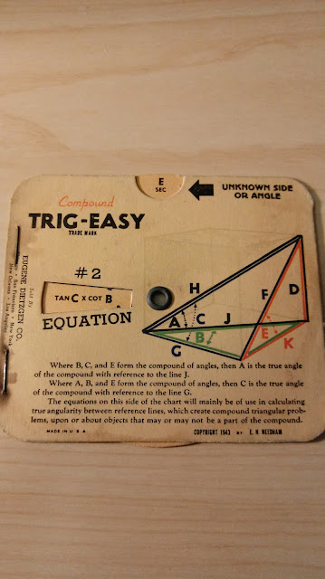
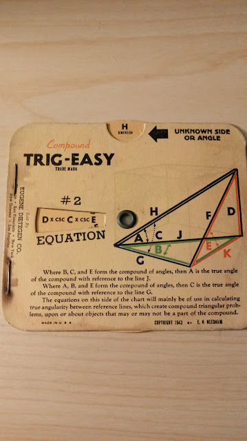
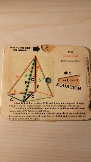
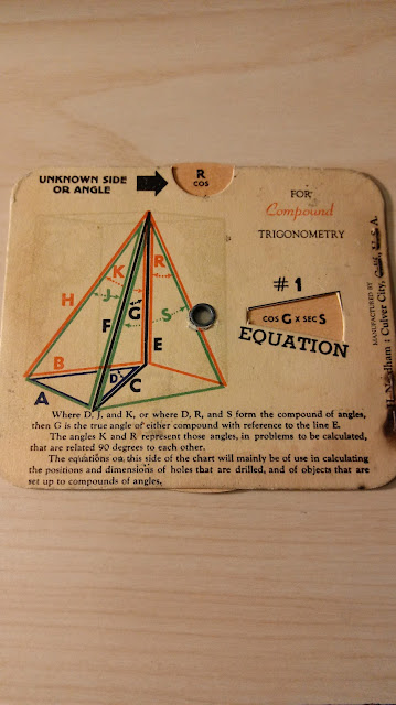
I purchased this cool, vintage formula card on Esty from the Lost Angeles Vintage Co. in Wofford Heights, California.  

The Compound Trig-Easy calculator is a 1943 formula reference card for calculating angels and lengths (dimension) of right triangle pyramids and rectangular pyramids.  Following are some example calculations.   

sec E = tan C * cot B

H = D * csc C * csc E

tan D = sin J * csc S

cos R = cos G * sec S

Eddie

All original content copyright, © 2011-2022.  Edward Shore.   Unauthorized use and/or unauthorized distribution for commercial purposes without express and written permission from the author is strictly prohibited.  This blog entry may be distributed for noncommercial purposes, provided that full credit is given to the author. 

Older Financial Calculators: Using the TVM Solver for LN(x) and EXP(x)

Older Financial Calculators:  Using the TVM Solver for LN(x) and EXP(x) 

Background and the Mathematics

Older and even some modern financial calculators do not have logarithm and exponential functions (ln, e^x).   However, the time value of money keys can be used to find exponentials and logarithms, as first mentioned by Hewlett Packard's HP-80 Application Note 80-007 (see Source below).  

Note the time value of money equation below:

FV = PV × (1 + I÷100)^n

where:

FV = future value  (Final)

PV = present value (1st Amt/Loan)

I = periodic interest rate (Int)

PMT = payment

n = number of payments (# pmts, term)

P/Y = 1   (set payments per year 1)

Let PV = 1.  Then:

FV = (1 + I÷100)^n

Let base = 1 + I÷100.  Then:

FV = base^n

And:

log_base(FV) = n 

log FV ÷ log base = n

Time Value of Money Setup

n = exponent

I = (base - 1) × 100

PV = -1*

PMT = 0

FV = (1 + I÷100)^n

For logarithm, enter FV and solve for n.

For exponentials, enter n and solve for FV. 

e^x, ln x:   set I = 171.8281828...

10^x, log x:   set I = 900

b^x, log_b(x):  set I = (b - 1) × 100

Examples

e^5.86 ≈ 350.7228

n = 5.86

I = 171.828

PV = -1  (+1 for calculators that do not follow the cash flow convention)

PMT = 0

Solve for FV

ln(376) ≈ 5.9296

I = 171.828

PV = -1  (+1 for calculators that do not follow the cash flow convention)

PMT = 0

FV = 376

Solve for n

Caution

This is works well for most financial calculators such as HP-80, HP 12C Classic, TI Personal Brother, Casio FC-100, Calculated Industries Qualifier Plus III FX 3430, and the HP 17BII+.  However, on some calculators, such as HP 12C Platinum, round calculations for n, so logarithm calculations will not be accurate.  

Source

Hewlett Packard.   HP-80 Application Notes:  Calculating Logs, Anti-Logs, And Roots of Numbers  No. 80-007.  December 10, 1973. 

Eddie

All original content copyright, © 2011-2022.  Edward Shore.   Unauthorized use and/or unauthorized distribution for commercial purposes without express and written permission from the author is strictly prohibited.  This blog entry may be distributed for noncommercial purposes, provided that full credit is given to the author. 

Binomial Expansion in Two Methods

Binomial Expansion in Two Methods

Expanding the Binomial by Two Methods

There are two ways to obtain the coefficients of expanding the binomial in the form (a ∙ x + b)^n:

1.  Binomial Theorem:

(a ∙ x + b)^n = Σ(comb(n, k) ∙ (a ∙ x)^k ∙ b^(n -k), k=0, n)

where comb(n,k) = n! ÷ (k! × (n - k)!)

2.  Maclaurin Series (Taylor series at point x=0):

f(x) = (a ∙ x + b)^n

f(x) =  f(0) + f'(0) ∙ x + f''(0)÷2! ∙ x^2 + f'''(0)÷3! ∙ x^3 + ... + f^n(0)÷n! ∙ x^n

Let's illustrate this through several examples.

Example 1:   (2∙x+3)^2

Binomial Theorem:

(2∙x+3)^2 

= comb(2,0)∙(2∙x)^2 + comb(2,1)∙(2∙x)∙3 + comb(2,2)∙3^2

= 4∙x^2 + 12∙x + 3

Maclaurin Series:

f(x) = (2∙x+3)^2,  f(0)=9

f'(x) = 4∙(2∙x+3), f'(0)=12

f''(x) = 8,  f''(0)=8

(2∙x+3)^2 = 9 + 12÷1! ∙ x + 8÷2! ∙ x^2 = 9 + 12∙x + 4∙x^2

Example 2:   (x + 5)^3

Binomial Theorem:

(x+5)^3

= comb(3,0)∙x^3 + comb(3,1)∙x^2∙5 + comb(3,2)∙x∙5^2 + comb(3,3)∙5^3

= x^3 + 15∙x^2 + 75∙x + 125

Maclaurin Series:

f(x) = (x+5)^3, f(0) = 125

f'(x) = 3∙(x+5)^2, f'(0) = 75

f''(x) = 6∙(x+5), f''(0) = 30

f'''(x) = 6, f'''(0) = 6

(x + 5)^3 = 125 + 75÷1! ∙ x + 30÷2! ∙x^2 + 6÷3! ∙ x^3 

= 125 + 75∙x + 15∙x^2 + x^3

Example 3:  A general binomial:  (a∙x+b)^2

Binomial Theorem:

(a∙x+b)^2

= comb(2,0)∙(a∙x)^2 + comb(2,1)∙(a∙x)∙b + comb(2,2)∙b^2

= a^2∙x^2 + 2∙a∙b∙x + b^2

Maclaurin Series:

f(x) =  (a∙x+b)^2, f(0) = b^2

f'(x) = 2∙(a∙x+b)∙a, f'(0) = 2∙a∙b

f''(x) = 2∙a^2, f''(0) = 2∙a^2

(a∙x+b)^2 = b^2 + (2∙a∙b)÷1! ∙x + (2∙a^2)÷2! ∙x^2 = b^2 + 2∙a∙b∙x + a^2∙x^2

 

Two ways of obtaining the expansion of the binomial.   

Eddie 

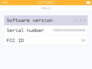
Numworks Update 17.2 - Highlights

 Numworks Update 17.2 - Highlights

Update is available at:

https://www.numworks.com/

The Numworks website will detect your calculator and will offer the update.

Here are some quick highlights:

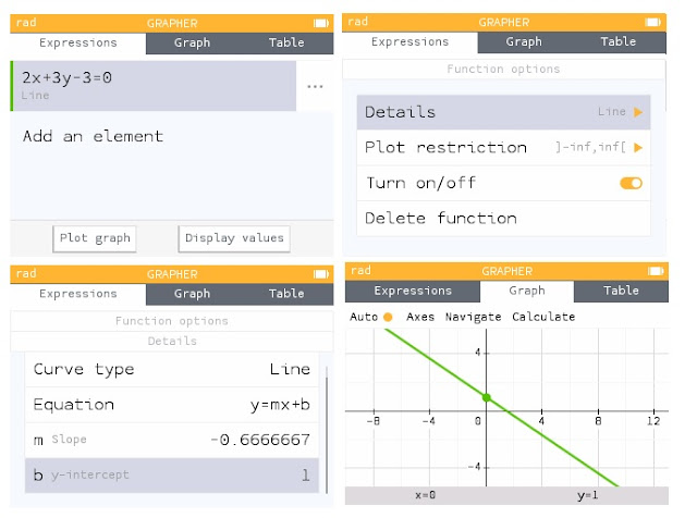
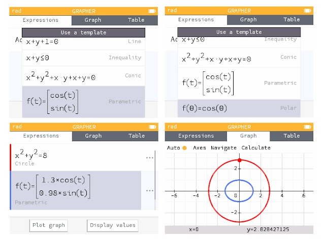
Extended graphing capabilities in Grapher.  In addition to functions f(x), lines, inequalities, conic sections, parametric equations, and polar equations can be graphed.  Different type of graphs can be plotted on the same screen.

Detail next to a line in Grapher (three dots) will display the slope and y-intercept.  Not pictured:  additional details added to Conic graphs.

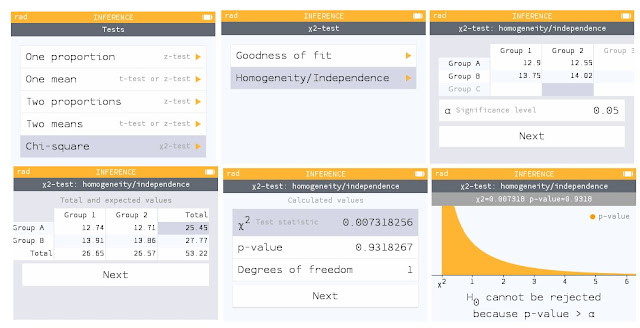
Major update to the Probabilities application, named Inference, includes tests and intervals.   Pictured here is a Chi-Square test of Independence.

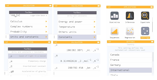
The toolbox contains scientific constants.  The units are determined by the Country setting in the Settings.  International is the SI units.   

The [ x, n, t ] cycles between x, n, t, and Θ.

For all the details (translation may be required):  https://www.numworks.com/calculator/update/version-17/

 

Eddie

All original content copyright, © 2011-2022.  Edward Shore.   Unauthorized use and/or unauthorized distribution for commercial purposes without express and written permission from the author is strictly prohibited.  This blog entry may be distributed for noncommercial purposes, provided that full credit is given to the author. 

HP 17BII+ and Numworks: Payment of a Loan with an Unusual First Period

 HP 17BII+ and Numworks: Payment of a Loan with an Unusual First Period

The First Payment Is Not Due in a Month

In finance, the first payment of a loan is not due at the end of a month from signing. This happens when all payments are due at a certain date, such as the 30th/31st or 1st of each month, regardless of when the loan papers are signed.  Loans of this type are referred to odd period loans or partial period loans.  Every payment after the first follows the conventional month time line.

HP 17BII+ Formula:  Partial Period Loan 

The following HP 17BII+ formula deals with calculating odd period loans.  This solver formula is directly from the HP 17BII+ Financial Calculator User's Guide, pg. 196 (see source):

ODD:  PV×(I%÷100×FP(DAYS÷30)+1)=-IF(DAYS<30:(1+I%÷100)×PMT:PMT)×UPSV(I%:N)-FV×SPPV(I%:N)

In the solver, the percent sign is a character used in variables, not a function.  PV, FV, PMT, I%, N are all valid variables in the HP 17BII+ solver.  The variables:

N:  number of payments

DAYS:  number of days in the first period, from 0 to 59.

I%:  the periodic interest rate.   For monthly payments, divide the annual interest rate by 12.

PV:  the loan amount

FV:  the balloon amount

PMT:  payment

This formula follows the cash flow convention:  negative amounts for cash outflows, positive amounts for cash inflows.

Numworks Script:  Partial Period Loan

oddperiod.py

My Numworks script:  https://my.numworks.com/python/ews31415/oddperiod

# 2021-11-14 EWS

# odd period

from math import *

print("Loan with partial period")

print("0 - 59 days")

print("Monthly Payments")

n=float(input("N: n? "))

rate=float(input("I/YR:  rate? "))

pv=float(input("PV: loan amt? "))

fv=float(input("FV: balooon pmt? "))

days=float(input("DAYS: odd period? "))

r=rate/1200

if days<30:

  j=1+r

else:

  j=1

f=days/30-int(days/30)

w=r*f+1

  

# uspv

u=(1-(1+r)**(-n))/r

# sppv

s=(1+r)**(-n)

pmt=(pv*w+fv*s)/(j*u)

# rounding

pmt=-int(pmt*100+.5)/100

# result

print("Payment: "+str(pmt))

Note:   the cash flow convention is followed

Examples

Loan 1:

Inputs:

N = 60

DAYS = 10

PV = $58,425.10

I%/YR = 4.48%  (annual rate), for the HP 17BII+, divide this by 12

FV = $0.00 (no balloon payment)

Result:  PMT:  -1,085.99  

Loan 2:

Inputs:

N = 240

DAYS = 40

PV = $16,956.00

I%/YR = 7.02%  (annual rate), for the HP 17BII+, divide this by 12

FV = $500.00 (enter -500.00 for HP 17BII+)

Result:  PMT:   -130.96

Source

HP 17BII+ Financial Calculator User's Guide.  Ed. 2.  Hewlett Packard.  San Diego, CA  2004

http://h10032.www1.hp.com/ctg/Manual/c00363348

All original content copyright, © 2011-2022.  Edward Shore.   Unauthorized use and/or unauthorized distribution for commercial purposes without express and written permission from the author is strictly prohibited.  This blog entry may be distributed for noncommercial purposes, provided that full credit is given to the author. 

HP 17BII+: Prorated Mortgage Interest and Prorated Property Tax

 HP 17BII+:   Prorated Mortgage Interest and Prorated Property Tax

Both formulas presented today are from Michael C. Thomsett's book, The Real Estate Investor's Pocket Calculator.  This book is excellent for real estate and financial mathematics.  Refer to the source section below.  The formulas are adopted for the HP 17B, 19B, and 27S families.

The follow formulas deal with prorated interest and property tax when property is sold.

Prorated Mortgage Interest

Calculate the amount of mortgage interest the buyer must pay upfront prior to the first payment of the mortgage.  

Solver Formula - HP 17BII+:

PROINT=LOAN×I%÷1200×PER÷MO

Variables:

PROINT:  prorated interest
LOAN:  mortgage amount
I%:  annual interest
PER:  number of days until 1st month the mortgage starts
MO: number of days in the month prior to when the mortgage starts

Example:

A mortgage closed on March 12, 2021, with the first mortgage month beginning April 1, 2021.  The mortgage is for $179,000 for 30 years (360 payments) at 2.76%.   What is the prorated interest the buyer must pay at closing?

LOAN:  179,000
I%: 2.76
PER:  19   (19 days until March 31, 2021)
MO:  31   (31 days in March 2021)

Result:   PROINT = 252.33

Prorated Property Tax

The formula calculates the prorated property tax the seller must pay when the mortgage is signed.  Often the property tax is assessed semi-annually.  

Solver Formula - HP 17BII+:

PROTAX=(DDAYS(BGN:SALE:1)+1)÷(DDAYS(BGN:END:1)+1)×$BILL

Variables:

PROTAX:  prorated property tax
BGN:  first day of the tax period
END:  last day of the tax period
SALE:  day when the mortgage closed
$BILL:  amount of the property tax

Example:  

Let's take the same scenario above, with the sale date of March 12, 2021.   The property tax for period January 1 to June 30, 2021 is $1,190.   

$BILL:  1,190
BGN:  1.012021  (MM.DDYYY format)
END:  6.302021
SALE:  3.122021

Result:  PROTAX = 466.80

Source

Thomas, Michael C. The Real Estate Investor's Pocket Calculator 2nd Edition.  AMACOM.  American Management Association:  New York. 2018  ISBN 9780814438893

All original content copyright, © 2011-2022.  Edward Shore.   Unauthorized use and/or unauthorized distribution for commercial purposes without express and written permission from the author is strictly prohibited.  This blog entry may be distributed for noncommercial purposes, provided that full credit is given to the author.

Casio fx-5800P: Lambert Function by Pierre Gillet

Casio fx-5800P: Lambert Function by Pierre Gillet

The programs on this blog entry are created and authored by Pierre Gillet. Gratitude for his permission to post this on my blog.

Introduction

The Lambert function is defined as:

    w = W(x) where  w * e^w = x

W(x) is the inverse of y = x * e^x: so, W(x) * e^(W(x)) = x and W(x * e^x)=x

In all cases, x must be >= -1/e to get a real value of W(x)

For x>=0, there’s only one value of W(x), called W0(x) (« principal branch »   of W(x))

For x<0, two values of W(x) are possible : W0(x) and W-1(x)

In all cases, W0(x) >= -1 and W-1(x) < = -1

The set of programs presented use W(x) to solve equations such as:

    x^x = a

    log x = x - 1

    a^x = b - x

where a and b are real constants.  

The trick to solve these kinds of equation is to transform them into the form

    f(x) * e^f(x) = constant

Then comes

    W(f(x) * e^f(x)) = W(constant)

    f(x) = W(constant) (remember that W(x * e^x) = x)

and then you normally solve easily for x but still have to calculate the above W(constant)

You can calculate W(p) (where p is constant) with the efficient Newton’s method solving the equation x * e^x – p = 0:

To get W0(p) : 

    if -1/e <= p <= 10 then x_0 = 0

    if p > 10  then x_0 = ln(p) – ln(ln(p))   (asymptotic behavior of W0(x))

To get W-1(p) :

    If -1/e <= p <= -0.1 then x_0 = -2

    if p > -0.1 then x_0 = ln(-p) – ln(-ln(-p))   (asymptotic behavior of W-1(x))

    Then iterate x_n = (x^2 + p * e^(-x)) / (x + 1)

      will normally converge to the desired W(p) value

See this post: 

https://math.stackexchange.com/questions/463055/approximation-to-the-lambert-w-function

Programs :

"W0FX"  // The program asks for x and displays W0(x) value (stored in W)

?X:0->G

X>10 => Ln(X)-Ln(Ln(X))->G

Prog "WSUB":W

"W-1FX"  // The program asks for x and displays W-1(x) value (stored in W)

?X:-2->G

X>-.1 => Ln(-X)-Ln(-Ln(-X))->G

Prog "WSUB":W

"WSUB"  // Subroutine called by W0FX and W-1FX

X<-e^(-1) => -1->G

10^(-10)->E:Lbl 1

(G^2+Xe^(-G))/(G+1)->W

Abs(G-W)<E => Return

W->G:Goto 1

Notes:

Precision is 1E-10 (see 10^(-10) in WSUB)

The first line in WSUB ensures Math error if X<-1/e

Note from Edward Shore:

?X is allowed on the fx-5800P:   When executed, the last value of X is shown which can be accepted or replaced.   It doesn't work for the Casio graphing calculators. 

Below is a graph of x*e^x vs. W_0 from W0FX and W_-1 from W-1FX, as created by the Desmos graphing app:

Examples

x^x = 2

    x * ln(x) = ln(2)    

    Let t = ln x (=>x = e^t)

    t * e^t = ln(2)

    W(t * e^t) = W(ln(2))

    t = W(ln(2))

    x= e^W(ln(2))

    Ln(2) is >= 0 => Only one value for W: on W0(x)

    Execute W0FX:

    Type ln(2) then EXE

    The program displays approx 0.4444 (ie W0(ln(2)))

    You are out of the program and now type e^(W)

    The machine displays approx 1.5596 (x value)

log x = x - 1

    x = 10^(x - 1)

    x = 10^x * 10^(-1)

    x = e^(x * ln(10)) * 10^(-1)

    x*e^(-x * ln(10)) = 10^(-1)

    -x * ln(10) * e^(-x * ln(10)) = -10^(-1) * ln(10)

    W(-x * ln(10) * e^(-x * ln(10))) = W(-10^(-1) * ln(10)

    -x * ln(10) = W(-10^(-1) * ln(10)

    x = -W(-10^(-1) * ln(10)) / ln(10)

    -10^(-1) * ln(10))) is < 0 => Two values for W : on W0(x) and W-1(x)

    Execute W0FX:

    Type -10^(-1) * ln(10) then EXE

    The program displays approx -0.3158 (ie W0(-10^(-1) * ln(10)))

    You are out of the program and now type -W / ln(10)

    The machine displays approx 0.1371 (first x value)

    Then Execute W-1FX:

    Press EXE (to keep the current value -10^(-1) * ln(10) in X)  (approx -0.2303)

    The program displays approx -2.3026 (ie W-1(-10^(-1) * ln(10)))

    You are out of the program and now type -W / ln(10)

    The machine displays approx 1 (second x value)

2^x = 11 - x

    Let t = 11-x (=>x = 11-t)

    2^(11 - t) = t

    2^11 * 2^(-t) = t

    2^11 * e^(-t * ln(2)) = t

    e^(-t * ln(2)) = t / (2^11)

    1 = t * e^(t * ln(2)) / (2^11)

    ln(2) = t * ln(2) * e^(t * ln(2)) / (2^11)

    2^11 * ln(2) = t * ln(2) * e^(t * ln(2))

    W(2^11 * ln(2)) = W(t * ln(2) * e^(t * ln(2))

    W(2^11 * ln(2)) = t * ln(2)

    t = W(2^11 * ln(2)) / ln(2)

    x= 11 - W(2^11 * ln(2)) / ln(2)

    2^11 * ln(2) is >= 0 => Only one value for W: on W0(x)

    Execute W0FX:

    Type 2^11*ln(2) then EXE

    The program displays approx 5.5452 (ie W0(2^11 * ln(2)))

    You are out of the program and now type 11 – W / ln(2)

    The machine displays approx 3 (x value)

What for numbers beyond 10^100 ?

Even for small values of the constants involved in an equation, you have        to calculate W(x) with rapidly astronomical arguments :

For example, with the equation 2^x = 1000 – x  (cf the 2^x = 11 – x case), you’d need to calculate W(2^1000 * ln(2)), causing overflow of most of the        calculators.

Here again, you can calculate W(p) (where p is constant) with the efficient        Newton’s method solving this time the equation ln(x) + x - ln(p) = 0, handling ln(p) instead of p:

To get W0(ln(p)): 

    x_0 = ln(p) – ln(ln(p))   (asymptotic behavior of W0(x))

Then iterate:  

x_n = x * (1 - ln(x) + ln(p)) / (x + 1)

will normally converge to W0(p)

Additional programs

"W0FLNX"  // The program asks for ln(x) and displays W0(x) value (stored in W)

?X:0->G

X-Ln(X)->G

Prog "WSUBLN":W

"WSUBLN"  // Subroutine called by W0FLNX

10^(-10)->E:Lbl 1

G(1-Ln(G)+X)/(G+1)->W

Abs(G-W)<E => Return

W->G:Goto 1

Notes:

If p is an excessively large number then W0FLNX asks for ln(p) and returns W0(p). Enter ln(p) in a good way : for example, not ln(10^1000) but 1000 * ln(10)

2nd line in W0FLNX: "X - Ln(X)" is in fact ln(p) - ln(ln(p)) since you entered ln(p) in X

Example

2^x = 1000 - x

    Solution : x = 1000 - W0(2^1000 * ln(2)) / ln(2) 

    (cf the Solve 2^x = 11 - x case)

    2^1000 * ln(2) is >= 0 => Only one value for W: on W0(x)

    2^1000 * ln(2) > 10^100 so you can’t execute W0FX

    Note that ln (2^1000 * ln(2)) = 1000 * ln(2) + ln(ln(2))

    Execute W0FLNX:

    Type 1000 * ln(2) + ln(ln(2))  then EXE

    The program displays approx 686.2494  (ie W0(2^1000 * ln(2)))

    You are out of the program and now type 1000 - W / ln(2)

    The machine displays approx 9.9514 (x value)

Thank you to Pierre Gillet.

Eddie 

All original content copyright, © 2011-2022.  Edward Shore.  Programs provided by Pierre Gillet with permission, © 2022.   Unauthorized use and/or unauthorized distribution for commercial purposes without express and written permission from the author is strictly prohibited.  This blog entry may be distributed for noncommercial purposes, provided that full credit is given to the author. 

Review: Calculated Industries 4090 Sheet Metal/HVAC Pro Review

Review:  Calculated Industries 4090 Sheet Metal/HVAC Pro Review 

Quick Facts

Model: 4090 Sheet Metal/HVAC Pro 

Company: Calculated Industries

Years: approx. 2004 - Present*

Memory Register:  1 independent memory, 3 general memory registers

Battery:  2 x LR44 batteries

Screen:  8 digits with alpha numeric prompts, 12 digit accuracy

Logic:  AOS (Algebraic), Chain 

Price:   retails about $89.95; iOS and Android app available for $29.99; used calculators can be found for less 

Web Page from Calculated Industries:  https://www.calculated.com/mobile/prd722/Sheet-Metal-HVAC-Pro.html

If you purchase it out of the box, either by repackage or retail, both an Armadillo Case and a hard slide cover come with the calculator.  In the box set has a full user's manual, which is really nice and gives an extensive amount of examples and details.  

History

The Sheet Metal/HVAC Pro was exclusive to the International Training Institute (ITI)(https://www.sheetmetal-iti.org/) until 2021, when Calculated Industries made the calculator available to the Public  (7 seconds into this video:  https://www.youtube.com/watch?v=wzmB8UAEjls).

I purchased a used Sheet Metal/HVAC Pro which is why you see the ITI logo in the pictures.  I am very confident both versions have the substantially the same amount of functions.  

Features

* Trigonometry and Right Triangles

* Square, Square Root, Cube, Cube Root

* Fan Laws

* Circle and Arc Calculations

* Column and Cone Calculations

* VP (velocity pressure)/FPM (feet per minute) conversions

* Offset calculations

* Stairs, Hip/Valleys, Jack

* And one of the best known features to come with Calculated Industries industry calculators:  feet-inch-fraction and meter-millimeter calculations. Fractions of inches can be set from 1/2" to 1/64".  I usually work with 1/16".  

I think this is the only calculator from Calculator Industries to have a exponent (10^xx) key (x 10^y), allow for numbers to be entered using scientific notation.  The maximum number is 9.999999 * 10^76.  

Trigonometry

The only angle unit the trigonometric functions work with is degrees.  Two unique features that come with the Sheet Metal/HVAC Pro are the ArcK constant and the Law of Cosines function.  

An ArcK constant, which is equal to π/180 ≈ 0.017453.  This constant is helpful for circle arc calculations.

The Law of Cosines function where given the lengths of three sides A, B, and C, calculate the angle measurements of each of the angle and the area of the triangle using Heron's formula.   This is one of my favorite features of the Sheet Metal/HVAC Pro, as going through the User Guide a lot of pipe work involves determining lengths and angles of triangles.  

There are four keys that deal with right triangles, the multi-purpose [ x (Run) ], [ y (Rise) ],  [ r (Diag) ], and [ θ (Pitch) ] keys.  Enter the given knowns and then just press the remaining keys to solve for the missing parameters.  

Fan Laws

The A and A new (which represent the CFM - cubic feet per minute), and the B and B new registers deal with the three fan laws.  The B and B new parameters change depending on which fan law is used.

Fan Law 1:  B and B new represent RPM (revolutions per minute)

Fan Law 2:  B and B new represent SP (static pressure)

Fan Law 3:  B and B new represent BHP (brake horsepower)

Stairs and Roofs

The Sheet Metal/HVAC Pro has the stair, hip valley, and jack rafter calculations, the same as the construction calculators Construction Pro 5 and the Construction Master Pro.   You can set the default riser height of the stairs, as well as calculate the number of required risers, stairs, the tread width, the stringer length.  The HVAC Pro also works with roofs:  rafter length, pitch, jack rafters including irregular jacks.  

Offset Calculations

The offset calculations on the Sheet Metal/HVAC Pro slightly differ from the offset calculations offered on the Pipe Trades Pro.  The offset deal with sheet metals, and the calculations included are:

*  centerline radius

*  wrapper length

*  throat and heel radius

Verdict

As always, Calculated Industries offers quality calculators that are specific to industrial needs and the Sheet Metal/HVAC Pro is no exception.  The key quality is great, the display has helpful prompts, and the Armadillo cases given solid protection.   I'm happy that this calculator is now available to the public.

Eddie 

All original content copyright, © 2011-2022.  Edward Shore.   Unauthorized use and/or unauthorized distribution for commercial purposes without express and written permission from the author is strictly prohibited.  This blog entry may be distributed for noncommercial purposes, provided that full credit is given to the author. 

Lines with Opposite-Signed Slopes

 Lines with Opposite-Signed Slopes

Take two lines, each with opposite signed slopes.  One slope has a positive slope, the other has a negative slope.   In general, the pair of lines will always intersect at one point.

Define two lines as such:

y = m1 ∙ x  + b1,  where m is the slope and b is the y-intercept.   

y = m2 ∙ x + b2

Assume that m1 and m2 are not zero, and m1 > 0 and m2 < 0.

If m2 < 0, -|m2| < 0  (see Aside) 

and as a result, m2 = -|m2|   

Also,  since m1 > 0, |m1| > 0, and m1 = |m1|.   

Equating both lines and solving for x:   

m1 ∙ x + b1 = m2 ∙ x + b2

|m1| ∙ x + b1 = -|m2| ∙ x + b2

|m1| ∙ x + |m2| ∙ x = b2 - b1

x = (b2 - b1) ÷ (|m1| + |m2|)

Since m1 and m2 are not zero, the above solution is defined.   

QED

- - - - - - - - - --  - 

Aside:    If x < 0, then  -|x| < 0  

Assume x is not zero. 

By definition, the absolute value of x, denoted as |x|, is the defined as the distance x is from 0 and is always positive. 

Then:

|x| > 0 

Multiply both sides by -1:

-|x| < 0

- - - - - - - - - --  - 

Eddie

All original content copyright, © 2011-2022.  Edward Shore.   Unauthorized use and/or unauthorized distribution for commercial purposes without express and written permission from the author is strictly prohibited.  This blog entry may be distributed for noncommercial purposes, provided that full credit is given to the author. 

Casio fx-3650P and fx-CG50: Partial Fraction Decomposition

Casio fx-3650P and fx-CG50:   Partial Fraction Decomposition

Casio fx-3650P (II) Program: Partial Fraction Decomposition

The following program calculates the coefficients decomposition, X and Y, as follows:

(A ∙ t + B) ÷ ((t + C) ∙ (t + D)) = X ÷ (t + C) + Y ÷ (t + D)

Note:  C ≠ D

where:

X = (B - A ∙ C) ÷ (D - C)

Y = A - X

Program:  (35 Steps)

? → A : ? → B : ? → C : ? → D : 

( B - A C ) ÷ ( D - C → X ◢ A - X → Y

Example:  

(2t - 3) ÷ ((t - 1)(t + 4))  = -0.2÷(t-1) + 2.2÷(t + 4)

A = 2, B = -3, C = -1, D = 4

Result:  -0.2, 2.2

The above algorithm should be good for the fx-7000G, fx-50FII, fx-4000P, fx-5800P, and other programming and graphing calculators (modifications may be necessary).

Casio fx-CG50 Program:  PARTFRAC

The code listed will also be good for the fx-9750G/fx-9860G series.

The program PARTFRAC, 720 bytes, will execute partial fraction decomposition of any of the three types:

(1)    (A ∙ x + B)÷((x + C) ∙ (x + D)) = R÷(x + C) + S÷(x + D)

Inputs:  A, B, C, D

Outputs:  R, S

[[ R ] [ S ]] = [ [ D, C ] [ 1, 1 ] ]^(-1) ∙ [ [ B ] [ A ] ]

(2)  (A ∙ x^2 + B ∙ x + C)÷((x + D)^2 ∙ (x + E)) = R÷(x + D)^2 + S÷(X + D) + T÷(x + E)

Inputs:  A, B, C, D, E

Outputs:  R, S, T

[[ R ][ S ][ T ]] = [[ E, D ∙ E, D^2 ][ 1, D + E, 2 ∙ D ][ 0, 1, 1 ]]^-1) ∙ [[ C ][ B ][ A ]] 

(3)  (A ∙ x^2 + B ∙ x + C)÷((x+D)∙(x+E)∙(x+F)) = R÷(x+D) + S÷(x+E) + T÷(x+F)

Inputs:  A, B, C, D, E, F

Outputs:  R, S, T

[[ R ][ S ][ T ]] = 

[[ E ∙F, D ∙ F, D ∙ E ][ E+F, D+F, D+E ][ 1, 1, 1 ]]^-1) ∙ [[ C ][ B ][ A ]] 

Program Listing:

'ProgramMode:RUN

"2021-11-05 EWS"

"PARTIAL FRACTION"

"N(X)/D(X)"◢

Lbl 0

Menu "DENOMINATOR?","(X+C)(X+D)",1,"(X+D)_^<2>_(X+E)",2,"(X+D)(X+E)(X+F)",3,"EXIT",E

Lbl 1

"(AX+B)/((X+C)(X+D))"◢

"A"?->A

"B"?->B

"C"?->C

"D"?->D

[[D,C][1,1]]^<-1>*[[B][A]]->Mat A

Mat A[1,1]->R

Mat A[2,1]->S

"=R/(X+C)+S/(X+D)"◢

"R="

R◢

"S="

S◢

Goto 0

Lbl 2

"(AX_^<2>_+BX+C)/((X+D)_^<2>_(X+E))"◢

"A"?->A

"B"?->B

"C"?->C

"D"?->D

"E"?->E

[[E,D*E,D^<2>][1,D+E,2*D][0,1,1]]^<-1>*[[C][B][A]]->Mat A

Mat A[1,1]->R

Mat A[2,1]->S

Mat A[3,1]->T

"=R/(X+D)_^<2>_+S/(X+D)+T/(X+E)"◢

"R="

R◢

"S="

S◢

"T="

T◢

Goto 0

Lbl 3

"(AX_^<2>_+BX+C)/((X+D)(X+E)(X+F))"◢

"A"?->A

"B"?->B

"C"?->C

"D"?->D

"E"?->E

"F"?->F

[[E*F,D*F,D*E][E+F,D+F,D+E][1,1,1]]^<-1>*[[C][B][A]]->Mat A

Mat A[1,1]->R

Mat A[2,1]->S

Mat A[3,1]->T

"=R/(X+D)+S/(X+E)+T/(X+F)"◢

"R="

R◢

"S="

S◢

"T="

T◢

Goto 0

Lbl E

"DONE."

Download (fx-CG 50):

https://drive.google.com/file/d/1hAIFrlX6xLMYPRiLz_dt7hpiP64CxmKC/view?usp=sharing

Examples To Try:

Type 1: 

(8 ∙ x + 3) ÷((x + 4) ∙ (x - 6))  = (29/10) ÷ (x + 4) + (51/10) ÷ (x - 6)

Type 2:

(x^2 + 4 ∙x + 5) ÷ ((x - 3)^2 ∙ (x + 1)) = 

(13/2) ÷ (x - 3)^2 + (7/8) ÷ (x - 3) + (1/8) ÷ (x + 1)

Type 3:

(2 ∙ x^2 + 3 ∙ x - 1) ÷ ((x - 1) ∙ (x + 2) ∙ (x + 4)) = 

(4/15) ÷ (x - 1) + (-1/6) ÷ (x + 2) + (19/10) ÷ (x + 4)

Eddie 

All original content copyright, © 2011-2022.  Edward Shore.   Unauthorized use and/or unauthorized distribution for commercial purposes without express and written permission from the author is strictly prohibited.  This blog entry may be distributed for noncommercial purposes, provided that full credit is given to the author. 

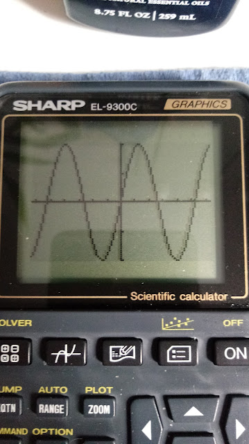
Retro Review: Sharp EL-9300C

Retro Review:  Sharp EL-9300C 

Quick Facts

Model: EL-9300C

Company: Sharp

Years: 1995 - 2000s  

Type:  Graphing with Programming

Memory:  23,064 bytes (programming, statistics, graph database, solver equations)

Battery:  4 AAA batteries, with 1 CR 2032 backup

Logic:  Algebraic, textbook

Comes with hard case.  The calculator I purchased came had in it's original box and manual.

The EL-9300C is part of the Sharp EL-9200/9300 family.   The earlier EL-9200/EL-9200C, released in 1992, had only 1,800 bytes.   I'm not sure about the difference between the EL-9300 and the EL-9300C.  The average cost of the EL-9300C is relatively inexpensive, around $15 to $25 U.S. dollars.  

Features

*  Mathematics with Calculus 

*  Complex Numbers Mode

*  Matrices

*  Base Mode

*  Graphing:  Function, Polar, Parametric

*  Equation Solver

*  Programming - up to 99 titled programs

*  Statistics with Linear Regression

*  Statistic Graphs with regression of six different regression fits

Mathematics with Calculus 

The EL-9300C (and its graphing family) has a rich set of scientific functions including numerical calculus.  The calculus functions include numeric derivative and numeric integral.

The numeric derivative works on functions in terms of X using the standard definition of the derivative:

f'(x) = (f(x+h) -f(x)) / h,  where h can be designated as an optional argument.   

The numeric integral uses to commands:   ∫ and dx.   The dx must be attached to the end unless an error occurs.  The integral uses calculates the Simpson's Rule   The number of subdivisions can be entered.  It is an early graphing calculator, so expect the calculator to take a few seconds to calculate integrals.  

Unfortunately, simplification of square roots and multiples of π are not included.   The EL-9300 still has fractions and fraction simplification.  

Complex Numbers Mode

For the time, the EL-9300 offers one most expansive set of pre-programmed calculations for complex numbers, which included logarithmic, power, exponential, trigonometric, and hyperbolic functions.  In trade, there the mantissa is 8 digits instead of the normal 10, and the complex mode is still separate.  

Matrices

Matrices are available, but they are in a separate mode.   Matrices are edited, created, and deleted through the MENU key, while called up by using the "mat" suffix through the MATH-E-1 keystrokes.

Basic row operations, inverse, transpose, and determinant.  

Base Mode

Base mode that allows logic operations for decimal, binary, hexadecimals, and octal integers are offered.  

Regardless of display mode, all matrices are show by the matrix's columns.  

Graphing:  Function, Polar, Parametric

The EL-9300C has three graphing modes, accessed through the SET UP menu.  If the calculator is in text mode, the function screen only displayed one equation at a time.  The graphing speed is fairly decent.  

Equation Solver

The solver is advanced, allowing for multi-character variables.  There are three methods:  Equation (where exact methods are used when available), Newton (using Newton's Method), and Graphic method.  

Newton's Method:  x_n+1 = x_n - f(x_n) ÷ f'(x_n)

Each equation can be saved and loaded into memory.  

Note, the equation solver is not available on the EL-9200.  

Programming 

The programming model is a basic version of basic.  Like the Equation Solver, multi-character variables are allowed.   There is a basic set of graphing commands.  The Input command included an automatic prompt.  For example:

Input base  returned  base? 

The automatic prompting will require getting used to.  

Loops, both conditional and unconditional, are handled by the use of Goto and Label.  

The EL-9300 can store up to 99 named programs.

The mode (Real, Matrix, N-Base, Complex) must be determined prior to creating a program.  Unfortunately, I have no way to change the SET UP in the program, such as fix settings, angle mode, and coordinate/graphing mode, we have to keep this mind.  

Statistics 

The statistics mode uses an index card interface.   There are four entry modes:

*  one variable

*  one variable with weights

*  two variable

*  two variable with weights

There is a one set of data and it must be cleared through the Delete Data (or Delete All) through the OPTION menu.  Statistical data can be calculated and graphed.  The EL-9300C offers up to six regression models (see below), but unfortunately, they are only available in graphing mode:

1.  y = a + b ∙ x   (linear)

2.  y = a ∙ e^(b ∙ x)  (exponential)

3.  y = a + b ∙ ln x  (logarithmic)

4.  y = a + b ∙ log x (common logarithmic)

5.  y = a ∙ x^b   (power)

6.  y = a + b ∙ x^-1  (inverse)

Common logarithmic is very unique, probably only offered on the EL-9200, EL-9300, and EL-9600 series.  

In calculation mode, we only have linear regression.  

One really cool feature of the Statistics mode, which will most likely not be able to found anywhere else is the ability to mask data.   A masked data point turns that data point "off", temporarily excluding the data point from calculation.  

Verdict

I like the perks of the EL-9300:  the ability to mask data points in statistics, extensive set of complex number commands,  the ability to save equations and use multi-character variable names (especially when most graphing calculators allowed only one-character variables, mainly A-Z and θ).  

However, be prepared to use separate modes for matrices, complex numbers, and general calculations (real mode).   The lack of set up commands in program will provide a challenge, and have to be set prior to running the programs.  

For the price, I find that the calculator is a good buy.  

Eddie

All original content copyright, © 2011-2021.  Edward Shore.   Unauthorized use and/or unauthorized distribution for commercial purposes without express and written permission from the author is strictly prohibited.  This blog entry may be distributed for noncommercial purposes, provided that full credit is given to the author.