Thursday, September 26, 2013

HP Prime Tip: Setting Up User Keys

HP Prime User Keyboard Primer

On of the features of the new HP Prime is the ability to assign custom programs, mathematical commands, or constants to the keyboard.

In this tutorial, we will use the shortcut commands to set up a user keyboard. You can set one or many user keys, there is no required number. In addition, the user keyboard can take one of four planes:

Key
Shift + Key
ALPHA + Key
Shift + ALPHA + Key

We will illustrate the procedure by assigning the STRING() command to the
Change Sign [ +/- ] key.

1. Create a new program and give it any name you want. For this example, I name the program USERKEY. USERKEY is going to be where I store my user key assignments.

2. Clear the program editor. There should be no EXPORT-BEGIN-END structures on the screen.

3. Press the [Menu] key. The [Menu] key is on the upper right hand corner section of the keys, to the left of the [CAS] key and below the [View] key. Select option 4: "Create User Key".

4. At the "Press any key..." prompt, select the key for which you want to assign your command to.

For my illustration, I will press the [+/-] key.

5. The user key template will appear of the programming editing screen. In between the BEGIN and END; is where you will type.

Note that the appropriate key code will be entered for you.

6. Call the RETURN command by pressing the soft key (Tmplt) then selecting "Block" then "RETURN".

Type your command and program in quotes. You can also call them from the various HP Prime menus or the Catalog. It is very important that you end this line with a semicolon (;), otherwise a syntax error occurs.

Note that user key assignments and edits are saved automatically. There is no need to run the USERKEY program.

Illustrated below is me putting the STRING() command. This assigns the STRING command to the [ +/- ] key.

For additional key assignments, repeat steps 3-6. Each key assignment template stands alone. Do not nest key assignment templates.

To use a user-assigned key, first press [Shift] + [Help] (User). An orange "1U" indicator appears on the top left hand corner of the screen. This means the next key pressed will execute the user-assigned function (if there is one).

For my example, pressing [Shift] + [Help] (User), [+/-] brings up the STRING command.

That is all there is to it!

Be sure to take notes of your key assignments.

Look for additional HP Prime programming tutorials in the upcoming months.

As always thank you for your support and comments. Have a great day everyone,

Eddie


This blog is property of Edward Shore. 2013

Sunday, September 22, 2013

HHC 2013 - Day 2 Highlights

The Morning Panel

The morning started off with a Q&A panel. The speakers were Ruth Patterson, Jason Smith, Cyrille de Brebisson, and Tim Wessman of the HC Calculator Group.

* The education market was a primary topic of the session, and how HP calculators, such as the Prime and 39gii, along with connectivity software play a role in education.
* The contrast of the keys and keyboard were discussed and how important it is to the user in terms of readability and usability. Note that most HP calculators the color of the type on the keys are black or white for the primary functions, and blue and orange for the shifted functions.
* There was a discussion of how the calculators can be used in both educational and professional settings.
* The HP Prime was named as such because the team wanted a mathematical term for a name, and to differentiate it from prior calculators which had numerical names.

At the end of the session the HHC committee presented two plaques: one to Cyrille de Brebisson for 15 years of being part of the calculator community and innovation, and one to Tim Wessman for 10 years.

David Ramsey - HP 85

David Ramsey talked about the HP 85 computer, and it is a beauty. Manufactured in 1980, the 85 had 16K of RAM that could be expanded to 64K. Only catch was up to 32K could be used for programming. It is a stand alone machine complete with printer. The screen is a 256 x 192 monochrome screen.

Plotting is limited on the HP 85; the pen could draw the axis, tick marks, lines, and points. However graphic buffers can be saved and restored. Processing can slow due to the limited amount of pins in the processor. The tape drive originally ran on DIC 100 cassettes, which had a limited life. Ramsey had his HP 85 modified so that QIC tapes are used. The back of the 85 had four ports, which a port can hold a drawer holding up to 6 ROM cartridges.

Calculators Are Awesome

Dan McDonald (I hope I get his name right, apologies if I don't) stated he like calculators because they are like puzzles and use allowed the our brains to be exercised. Namir Shammas commented that calculators are accessible devices. I agree with both gentlemen.

Readable 41 Bar Codes & Programs

Jake Schwartz and Jackie Woldering showed a project they completed. Everyone at the conference received two DVDs:

* A four-volume set of notes from previous PPC conferences, calculator journals, conference proceedings from Australian conferences, notes from all of the previous HHC conferences, and HP 41 programs, 1,343 programs consisting of 5,844 pages, complete with bar codes and dot data files. We thank both Jake and Jackie for hours and hours and hours of hard work, typing, and dedication to this project.
* A DVD of 1970s calculator ads.

Charles McCord: Life at HP

Charles McCord (again, apologizes if I have the name wrong) spoke about his life working at Hewlett Packard. He was inspired to save money over the last two years of high school and some of the first year in college to purchase a HP 65 after his father bought a HP 45, and how to understand how calculators work.

When working for HP in Corvallis, McCord started as a quality engineer working with the HP 41. He lead a team develop a modem for the HP 75, which gave it additional memory and power, at the request of AT&T. He was also a manager for the single chips produced for the HP 10 series. McCord also lead a group of engineers to develop printers and mini-computers in Vancouver and San Diego.

Some funny antidotes during his time at HP were:

* One of his supervisors was humorously given an HP 41C glued to a car battery since heavy ROM use easily ate up the battery.
* The first modem cases for the HP 75 were fine except the computers were resetting. Turns out the case pressed the keys for a soft reset. Plastic shields that were added to the case took care of the problem.
* In a test group for the original HP 12C, one of the NAND gates were locked, causing a row of commas to fill the screen each time the ON and decimal point keys were simultaneously pressed. Those calculators were not sold.
* People returned their otherwise working HP 12Cs after several years of use because the batteries lasted so long, they did not realize that the batteries died.

McCord now works for Aptima.

Final Panel, Prizes, and a Tour

A final panel assembled by Joe Horn, Cyrille de Brebisson, Jeremy Smith, Goeff Quickfall, Wlodek Mier-Jędrzejowicz, and Jim Donnelly takes about the adventures and misadventures of publishing.

Contest Winners:

Best Speaker, as voted by the attendees, went to Geoff Quickfall.

RPN Programming Contest Winner: Eric Smith

RPL Programming Contest Winner: Bill Butler

Congratulations to all the winners. I believe you can find details of the RPN and RPL contests on the HHC 2013 page and the HP Museum of Calculator Forum.

Of course, no conference is not complete with door and premium prizes. And there was enough to go around for all 56 attendees at least once. It was by random drawing and whoever gets called gets a choice of donated goodies. Here is what I won:

An HP 38G (1995). This is the beginning of the 38G/39G/40G/Prime family. Thanks to whoever donated the calculator.

For the record, I took two slide rules and printed two dairies of HP calculator programs that I wrote for various calculators.

Then there are the premium prizes, those donated items deemed by the community to be very valuable and/or unique. While I wasn't lucky enough to win a premium prize (but that is how I won my HP-71B two years ago) some of the premium prizes were:

* HP 65 in its box with accessories
* HP 75 in its box with accessories
* HP 25 with its charger and pouch. A good iOS emulator is the GO-25.
* HP 71-B
* HP 15C Limited Edition in its box, unopened (2)
* HP 48GX with a black LCD screen. 48GX calculators with black LCD screens are rare because they were the last 48GX to be produced. Most 48GX (and 48s in general) have blue LCD screens.
* Microsoft Surface Tablet
* HP calculator carrying case (2)

I am not sure if the names of the winners are posted on the HHC 2013 web site.

Tim Wessman took a group of us on a tour of the office, where testing of calculators and connectivity software takes place.

I had to leave to get to my hotel to connect for my ride to the airport. I probably have missed out on closing remarks and the after-conference party. I have to be back to work the following Monday.

Once again, my heartfelt gratitude to all the attendees and the committee, a lot who have become friends, and to Hewlett Packard. You are a big reason why math and calculators are lifelong loves for me.


Another conference has come and gone. Had a blast as always. Time flies when we are having fun. And I will talk to you next time!

Eddie


This blog is property of Edward Shore. 2013

Saturday, September 21, 2013

HHC 2013: Day 1 Highlights

First of all, thanks to Hewlett Packard and everyone at the HHC 2013 committee (http://hhuc.us/2013/committee.htm) - you are all amazing!

What a long, fun, and intense day. Here are some of the highlights from today:

The HP Prime Has Arrived!

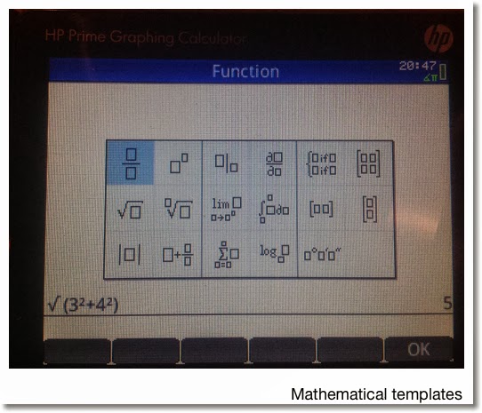
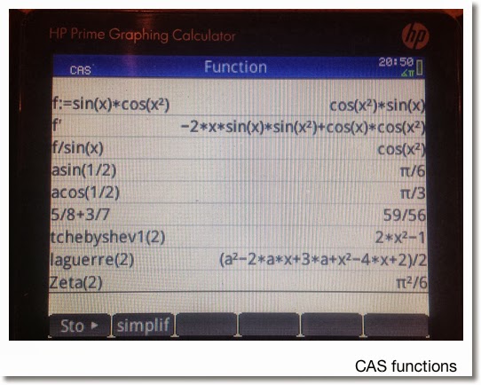
The new HP Prime is available! Prime, I believe is HP's first color graphing calculator. Features include a computer algebra system mode (CAS), graphing which includes geometry including slope-fields of differential equations, equation solver, full operational touch screen including finger scrolling and selecting, a spreadsheet application, and my favorite new feature: advanced graphing (color implicit graphing)! Below are pictures of the Prime:

Some more specifics:

* Super advanced functions including the special functions Gamma, Beta, Zeta, Si, Ci, Psi, and Error.
* Polynomials functions include Hermite, Lagrange, Laguerre, Legendre, Chebyshev, Cyclomotic, and Groebner.
* The programming language is similar to the programming of the HP 39gii and 39gs.
* Rechargeable battery with indicator.
* 240 x 320 full color pixel screen.
* App structure similar to the HP 38G/39G family. (And 40G for those living outside the United States).
* The connectivity kit is dynamic, you can update the calculator and the emulator in real time.
* RPN mode.
* Intelligent, multi-use programming commands.
* Battery life lasts a good long time, I am told up to 23 days under normal use. Of course, use varies is dependent on how intense the calculation is used.

Where can I get one? So far hpcalc.org, Bach Company, Samson Cables, and yes, even eBay has calculators for sale. Availability varies.

How much does the Prime cost? Approximately $130 to $150 (U.S. dollars).

I am looking to work with several of my friends and HP calculator enthusiasts on a Wiki page. Details are coming soon. And of course, I will be talking a lot more about Prime on this blog as well.

We spent three hours without blinking talking about Prime this morning with Tim Wessman and Cyrille de Brebisson.

Once again, thanks to all the speakers. It is one of my goals to actually have a presentation next year.

Jim Donnelly: Visualizing Data: A Journey From Calculator Development to the Machine Shop

Jim is the author of the several books on HP Calculators, including the "HP 48 Handbook". His contributions include adding drawing peripherals to classic HP calculators, the HP-71B Data Acquisition Pac, the Periodic Table for the HP 48G Series, and gave the legendary HP-01 calculator watch a new tool: a battery door opener. Jim also engraves designs and lettering onto aluminum plates, which includes a cryptic engraving "6accdae13eff7i3l9n4o4qrr4s8t12vx". It has something to do with calculus.

Other Highlights

Jim Johnson, from. Indianapolis, restored a HP-29C from a dead calculator to a full working one. He detailed how he took the calculator apart, cleaned the keyboards, gave it new batteries, and diagramed the electronics of the calculator.

Tip: Do not plug a Woodstock calculator (HP 21 to HP 29, 1970s) unless it had a good battery. Otherwise, the battery may get fried.

Namir Shammas highlighted some of his favorite functions of the HP Prime: extensive random number generators, advanced mathematical functions, and matrix factorization. His article can found in the September 2013 of HP Solve. (http://h20331.www2.hp.com/hpsub/downloads/hp_calculator_enl_sep_2013_v4.pdf)

Eric Smith, who is on a mission to build a working RPN (Reverse Polish Notation) calculator from scratch. After several years of research he is able to pass around two working demos: one that emulates the HP-41 and one that emulates HP-42 (the latter by popular demand). Everything is open source. Smith is now working on how to get the SD card inserted into calculator and fully working. During his talk a poll was taken and the majority of attendees preferred AA batteries over AAA and button sized batteries.

Jeremy Smith brought new life to road dots. A road dot the small circular numb that lines the lanes on our streets. He had designed several spherical pieces using road dots. He has also constructed a folding block of sixteen half-cubes connected by a string and a folding chess board.

Wlodek Mier-Jędrzejowicz received an appreciation award for thirty years of contributions to the Hewlett Packard calculator community. Congratulations and well deserved!

Gene Wright brought his collection of HP OmniBooks, which were manufactured in the 1990s, for show and tell. OmniBooks started as small notebooks (EX: 300) and by the end of their production run, they were full laptops (EX: EX3). Wright's collection focused on the earlier models.

Some specs of the OmniBook 300:
* 20 MHz Processor
* 9" diagonal grayscale screen
* Windows 3.1 Operating System
* Microsoft Office built into the ROM
* HP Calculator Application: Runs like the HP 19B except with a full keyboard.
* The mouse lived inside the notebook, came out with a press of a button.

Wright's collection includes the OmniBook 600C and OmniBook 530, with a broken screen.

Geoff Quickfall, a pilot who flies internationally, showed his typical workday. He uses the following HP Calculators on his flight:
* HP01 for active its timer feature so the crew can tell its passengers when they will arrive at their destination. Also the dynamic time features allows him to calculate how much fuel is used.
* HP 71B for matching and verifying latitudes at certain points of the flight.
* HP 41C with memory module to estimate the distance between airports. Quickfall also programmed the longitude and latitude coordinates of airports he flies to. The 41C is also used to print and organize break schedules for the flight crew.
* HP 42S for to calculate the fuel left in the tank (by weight), and to see if the fuel levels passes standards.
* HP 67, 29C, and 48 G are also used

IMHO, I am a little jealous - I wish I could use one advanced calculator at my job on a regular basis. But accounting does not use mathematics beyond arithmetic 99.9% of the time.

The day closed with Wlodek Mier-Jederzejowick showing us his latest edition of "A Guide to HP Handheld Calculators and Computers".

There you have it - the highlights. I will report on Day 2, hopefully tomorrow.

Eddie

This blog is property of Edward Shore. 2013

HHC 2013

Greetings from Fort Collins, CO!

I am here at Fort Collins, CO attending the annual HHC (HP Handheld Conference 2013). Basically, this is what ComicCon would be for calculator enthusiasts, particularly calculators made by Hewlett Packard.

This is my sixth conference I had attended over the last decade. HHC is a two day conference taking place over the weekend. We usually fly/drive to our destination on Friday - meet and have dinner. There are some attendees who go on torus and field trips. Saturday is our intense day - we literally start from sunrise to at least 9:00 at night. Sunday is more relaxed, and that is where we have contests and door prize drawings.

The web site of the conference is: http://hhuc.us/2013/index.htm, which takes place this weekend. HHC takes place during September.

Over the weekend, if I am able to, I will relay some of the highlights. Until then, have a great day!


Eddie


This blog is property of Edward Shore. 2013

Saturday, September 14, 2013

My Calculated Industries Calculator Collection

The company Calculated Industries (http://www.calculated.com/) manufactures specialized calculators.

Here is my small collection:

Machinist Calc Pro

I bought this calculator today at a pawn shop in Pomona. It came with the box, instructions, and the calculator in an Armadillo Gear case. I never seen a calculator being in such an industrial case before. This calculator is specialized in machinery calculations with a built in tables of drill points, drill sizes, and thread sizes. Trigonometric functions are featured (Adj, Opp, Hyp, Angle for right triangles and Sine, Cosine, Tangent for general trigonometry).

The manual is a good size book and as of today I have yet to go through it and do the examples.

Qualifier Plus IIx

This calculator specializes in real estate calculations, which include finding qualified amounts, time value of money, and PITI (principal, interest, taxes, & interest). I picked up this calculator at another pawn shop in Pomona, which is sadly no longer there.

The next three calculators deal with construction.

ProjectCalc Plus

I think I got all three of construction calculators from Home Depot throughout last year.

First is the simple calculator. The calculator had built in tables for concrete, carpet, and tile sizes (and more).

Material Estimator

To me, the Material Estimator is the big cousin of the ProjectCalc Plus. The Material Estimator has all the features plus an electric tape to keep track of calculations, a hard cover that stores the manual (which is really neat), and it is solar and battery powered.

Construction Master 5

The Construction Master takes a different specialty than the ProjectCalc and Material Estimator. The Construction Master focuses on stairs, roofs, risers, and walls. Like the Material Estimator, the Construction Master has an electric tape and the manual is stored in the calculator's case.

What is common for all the construction calculators and the Machinist Calc is that we can make calculations using yards-feet-inch, meters-centimeters-millimeters calculations and conversions. This is a super feature.

I really could use some more time learning the features of these calculators. So there is my collection.

Eddie


This blog is property of Edward Shore. 2013


Friday, September 13, 2013

Differential Equations #12: Reduction of Order

Introduction

The general n-order differential equation


can be translated into a system of first-order differential equations:

For a second-order equation

y" + A*y' + B*y = f(x)

The system is

y'_1 = y_2
y'_2 = f(x) - A*y_2 - B*y_1

Now time for examples.

1. y" + 3*y' - 4*y = 2

Let y_1 = y and y_2 = y'_1. Then:
y_2 = y', and

y'_2 = y"
y'_2 = 2 - 3*y' - 4*y
= 2 - 3*y_2 - 4*y_1

So our system is:
y'_1 = y_2
y'_2 = 2 - 3 * y_2 - 4 * y_1


2. 3*y" + 6*y' = -9

Let y_1 = y and y_2 = y'. Then:

y'_1 = y_2
y'_2 = y"
3*y" = -9 - 6*y'
y" = -3 - 2*y'
y'_2 = -3 - 2*y_2

The system is:
y'_1 = y_2
y'_2 = -3 - 2*y_2


We can go the other way, from a system of linear differential equations to a single multi-order differential equation.

3. y'_1 = y_2
y'_2 = y_1 + y_2


Again, let y_1 = y and y_2 = y'. Then:
y'_2 = y_1 + y_2
y" = y + y'
y" - y' - y = 0

4. y'_1 = y_2
y'_2 = 2/7 * y_1 - 3/7 * y_2 + 1/7


With y_1 = y and y_2 = y',
y'_2 = 2/7 * y_1 - 3/7 * y_2 + 1/7
y" = 2/7 * y - 3/7 * y' + 1/7
y" + 3/7 * y' - 2/7 * y = 1/7
7*y" + 3*y' - 2*y = 1

This concludes this blog post of Differential Equations. In a week I will be headed to Fort Collins. CO for the HHC 2013 conference. I am so excited - may the bad weather go away and everyone be safe!

Eddie


This blog is property of Edward Shore. 2013

Monday, September 9, 2013

Differential Equations #11: Numerical Solutions with the Runge-Kutta 4th Order Method


Update:  One of the numerical example (example 1) has incorrect numerical results.  This blog has been edited.  The results posted are now correct. Apologizes. -  Eddie
1/4/2015

Introduction

In this blog we will explore one of the ways to solve the differential equation y' = f(x,y) by numerical methods. One of the common methods is the Runge-Kutta 4th Order Method, probably the most common methods.

With the initial condition (x_n, y_n) and step size h, the next point (x_n+1, y_n+1) is calculated by the following equations:
x_n+1 = x_n + h
y_n+1 = y_n + (k1 + 2*k2 + 2*k3 + k4)/6 with

k1 = h * f(x_n, y_n)
k2 = h * f(x_n + h/2, y_n + k1/2)
k3 = h * f(x_n + h/2, y_n + k2/2)
k4 = h * f(x_n + h, y_n + k3)

(Almost) obviously use either a calculator or mathematical software for this process.

Examples:
1. dy/dx = -0.23 * (y + 1)
Initial Condition: (0, 24)
We want y1 when x1 = 1 and y2 when x2 = 2.


Observe that h = 1 with x0 = 0 and y0 = 24. Note the lack of x term in f(x,y).

Then:
x1 = 0 + 1 = 1
k1 ≈ -5.75
k2 ≈ -5.08875
k3 ≈ -5.16479375
k4 ≈ -4.562097438
y1 ≈ 18.86346918

x2 = 1 + 1 = 2
k1 ≈ -4.568597911
k2 ≈ -4.043209151
k3 ≈ -4.103628858
k4 ≈ -3.624763273
y2 ≈ 14.78229631

So our points are:
(0, 24)
(1, 18.86346918)
(2, 14.78229631)


2. y' = y - x with I.C. y(0) = 2
Find y(0.1) and y(0.2).


Note h = 0.1 with x0 = 0, y0 = 2, and f(x,y) = -x + y.

x1 = 0.1
k1 = 0.1 * f(0, 2) = 0.2
k2 = 0.1 * f(0.5 * 0.1, 2 + 0.5 * 0.2) = 0.205
k3 = 0.1 * f(0.5 * 0.1, 2 + 0.5 * 0.205) = 0.20525
k4 = 0.1 * f(0.1, 2 + 0.20525) = 0.210525
y1 = 2 + (0.2 + 2 * 0.205 + 2 * 0.20525 + 0.210525)/6 ≈ 2.205171

x2 = 0.2
k1 ≈ 0.210517
k2 ≈ 0.216043
k3 ≈ 0.216319
k4 ≈ 0.222149
y2 ≈ 2.421203

So our points are:
(0, 2)
(0.1, 2.205171)
(0.2, 2.421203)


Talk to you all next time!
Eddie

This blog is property of Edward Shore. 2013

Sunday, September 8, 2013

Differential Equations #10: Critical Points

Critical Points and Determining What Happens

In this blog entry we are working with a system of two equations:

x' = f(x,y)
y' = g(x,y)

where x and y are functions of a independent variable, say t for example. Well treat t as a time variable.

Today's blog will cover a three step process:
1. Finding Critical Points
2. Determining the Jacobian Matrix
3. Finding the Eiegenvalues of that Jacobian Matrix

1. Finding Critical Points

It is relatively easy to find the critical points of a system. Add that needs to be done is to set x' = 0 and y' = 0. The next step is to solve for x and y.

2. Determining the Jacobian Matrix

The Jacobian matrix of the system is


Hint: If the system is
x' = Ax + By
y' = Cx + Dy

Then the system's critical point is (0, 0) and the Jacobian Matrix is

J = [ [A, B] [C, D] ]


3. Determine the Eigenvalues

As we recall the eigenvalues of a 2 × 2 matrix can be determined by solving the following characteristic equation:

λ^2 - trace * λ + determinant = 0

Where:
* trace is the sum of the matrix's diagonal elements
* determinant is the determinant of the matrix

The roots are crucial and determine the behavior of the critical point.

Types of critical points:
* source: individual curve solutions x(t) and y(t) are trajectories going away from the critical point
* sink: individual curve solutions x(t) and y(t) are trajectories go towards the critical point
* saddle point: the critical point acts as a sink for some trajectories and a source for other trajectories
* center: trajectories orbit around the critical point, most likely circular or elliptical orbits

Determining the type of critical points:
* λ1 and λ2 are real and positive: critical point is a source.
* λ1 and λ2 are real and negative: critical point is a sink
* λ1 and λ2 are real and have opposite signs: critical point is a saddle
* λ is a double root and it's positive: critical point is a source
* λ is a double root and it's negative: critical point is a sink
* λ = S ± Ti and S is positive: point is a source, trajectories are spiral
* λ = S ± Ti and S is negative: point is a sink, trajectories are spiral
* λ = ± Ti: critical point is a center

Source: http://kaharris.org/teaching/216/Lectures/lec28/lec28.pdf

Let's work with some examples.

1.
x' = x + 4y
y' = 2x + 3y


Critical Point:
0 = x + 4y
0 = 2x + 3y

x = -4y
0 = 2(-4y) + 3y which implies y = 0 and x = 0

Our critical point is (0,0). The Jacobian matrix is J = [ [1, 4] [2, 3] ].

trace(J) = 1 + 3 = 4
det(J) = 1 * 3 - 2 * 4 = -5

The eigenvalues are:
λ^2 - 4*λ - 5 = 0
(λ - 5)(λ + 1) = 0
λ1 = 5, λ2 = -1
Real and opposite signs, the critical point (0,0) is a saddle point.

2.
x' = x + 2y - 6
y' = 6x - 3y + 24


Critical Point:
0 = x + 2y - 6
0 = 6x - 3y + 24

Which leaves is with the system of
x + 2y = 6
6x - 3y = -24

Solving the system yields the critical point (-2, 4).

With
f = x + 2y - 6
df/dx = 1
df/dy = 2
g = 6x - 3y + 24
dg/dx = 6
dg/dy = -3,

The Jacobian matrix is
J = [ [1, 2] [6, -3] ]

The eigenvalues of J are 3 and -5. Since the eigenvalues are real and are of opposite signs, the critical point (-2, 4) is a saddle point.

3.
x' = 2x + 3y
y' = x - 2y^2


Finding the critical points:
0 = 2x + 3y
0 = x - 2y^2

x = 2y^2
0 = 2(2y^2) + 3y
0 = 4y^2 + 3y
0 = y * (4y + 3)
which implies that we have two critical points, one with y = 0 and the other with y = -3/4.

If y = 0, then x = 2*0^2 = 0. One critical point is (0,0).
If y = -3/4, then x = 2*(-3/4)^2 = 9/8. The other critical point is (9/8, -3/4).

With
f = 2x + 3y, df/dx = 2, df/dy = 3
g = x - 2y^2, dg/dx = 1, dg/dy = -4y

Critical Point (0,0):
J = [ [2, 3] [1, 0] ]
And the eigenvalues of J are -1 and 3.
The critical point (0,0) is a saddle point.

Critical Point (9/8, -3/4):
J = [ [2, 3] [1, 3] ]
And the eigenvalues are (5 ± √13)/2. Approximate values are 4.302776 and 0.697224. The critical point (9/8, -3/4) is a source.

Hope this helps and we'll talk next time. Please feel free to post questions and comments.

Eddie


This blog is property of Edward Shore. 2013

Wednesday, September 4, 2013

XOR vs Addition, AND vs Multiplication


Hi everyone!

In this blog post, all numbers with a "b" after them are designated binary numbers. (the extra zeroes in front are for illustration purposes only)

XOR vs Addition

The logical operator XOR and addition may be very similar, but they are not the same.

Examples:

1101b + 0110b = 10011b but 1101b XOR 0110b = 1011b
1001b + 0011b = 1100b but 1001b XOR 0011b = 1010b

Truth table for XOR (Exclusive OR):
1 XOR 1 = 0
1 XOR 0 = 1
0 XOR 1 = 1
0 XOR 0 = 0

XOR is like addition if we let 0 represent an even number and 1 represent an odd number:
odd + odd = even
even + odd = odd
odd + even = odd
even + even = even

AND vs Multiplication

Likewise, the logical operator AND and multiplication may be very similar, but they are not the same.

Examples:
1101b × 0010b = 11010b but 1101b AND 0010b = 0000b
1100b × 1110b = 10101000b but 1100b AND 1110b = 1100b

Truth table for AND:
1 AND 1 = 1
1 AND 0 = 0
0 AND 1 = 0
0 AND 0 = 0

And likewise, AND is like addition if we let 0 represent an even integer and 1 represent an odd integer:
odd × odd = odd
odd × even = even
even × odd = even
even × even = even

Hopefully this clears any confusion up between arithmetic and two logic gates sometimes labeled as arithmetic. As always, love any comments and thanks as always.

Eddie


This blog is property of Edward Shore. 2013

Properties of A^x + B^y = C^z with Jonathan Neal


During our study of the Beal Conjecture with my friend and fellow mathematics graduate Jonathan Beal, we looked at the equation

A^x + B^y = C^z

where A, B, C, x, y, and z are integers. As a result A^x, B^y, and C^z are integers.

Let A^x be even (where A is a multiple of 2). Let B = p*m where p is a prime number. Then B^y = p^y * m^y.

The only even prime is 2. All other prime numbers (3, 5, 7, etc. ) are odd.

So if A^x is even and
p = 2 and m is even: p^y is even, m^y is even, B^y is even, and C^z is even.
p = 2 and m is odd: p^y is even, m^y is odd, B^y is even, and C^z is even.
p ≠ 2 and m is even: p^y is odd, m^y is even, B^y is even, and C^z is even.
p ≠ 2 and m is odd: p^y is odd, m^y is odd, B^y is odd, and C^z is odd

Assuming A^x is odd and
p = 2 and m is even: p^y is even, m^y is even, B^y is even, and C^z is odd.
p = 2 and m is odd: p^y is even, m^y is odd, B^y is even, and C^z is odd.
p ≠ 2 and m is even: p^y is odd, m^y is even, B^y is even, and C^z is odd.
p ≠ 2 and m is odd: p^y is odd, m^y is odd, B^y is odd, and C^z is even.

Eddie


This blog is property of Edward Shore. 2013


Monday, September 2, 2013

Differential Equations #9: Solving x'(t) = f(y(t)), y'(t) = g(x(t))

Solving
x'(t) = f(y(t))
y'(t) = g(x(t))


Sometimes using algebra can be more efficient than using Laplace transforms in solving systems of differential equations.

Procedure - two paths we can take:

1. Take the derivative of x', x" = f'(y)
2. Solve for y' and equate it to g(x).
3. Solve for x(t).
4. Solve for y(t).

OR

1. Take the derivative of y', y" = g'(x)
2. Solve for x' and equate it to f(y).
3. Solve for y(t).
4. Solve for x(t).

Let's take some examples and see how this works. In all examples presented, x and y are functions of t.

1.
x'= 2y
y'= -2x


x" = 2y'

Solving for y':
y' = x"/2

Equate to g(x):
x"/2 = -2x
0 = x"/2 - 2x
0 = x" - 4x

We have a homogenous second order differential equation.

Characteristic Equation: λ^2 + 4 = 0
Roots: λ = ± 2i

Hence
x = C1 cos(2t) + C2 sin(2t)

Note x' = 2y.
y = x'/2
y = [d/dt C1 cos(2t) + C2 sin(2t) ] /2
y = -C1 sin(2t) + C2 cos(2t)

Solution:
x = C1 cos(2t) + C2 sin(2t)
y = -C1 sin(2t) + C2 cos(2t)


The practical approach to this type of problem is to end up working with a homogenous second order differential equation, if possible.

2.
x' = y + 1
y' = 2x


Note
x" = y'

Then
y' = x" = 2x
0 = x" - 2x

We have a homogenous second order equation where the characteristic equation is
λ^2 - 2 = 0 and λ = ±√2 (-√2 and √2).

So
x = C1 e^(√2 * t) + C2 * e^(-√2 * t)

With
x' = √2 * C1 * e^(√2 * t) - √2 * C2 * e^(-√2 * t) = y + 1
y = √2 * C1 * e^(√2 * t) - √2 * C2 * e^(-√2 * t) - 1

Solution:
x = C1 e^(√2 * t) + C2 * e^(-√2 * t)
y = √2 * C1 * e^(√2 * t) - √2 * C2 * e^(-√2 * t) - 1


If we run into a non-homogenous second order differential equation, its not the end other world, refer to Part 8 ( http://edspi31415.blogspot.com/2013/09/differential-equations-8-second-order.html) on how to deal with such equations.

The next example I purposely set it up so we are going to use variation of parameters.
3.
x' = y + 3
y' = -3x


Observe that y" = -3x' and x' = -y"/3, and

y"/3 + y + 3 = 0
y" + 3y + 9 = 0
y" + 3y = -9
y = y_h + y_p

y_h:
λ^2 + 3 = 0, λ = ± i*√3
y_h =C1 cos(t * √3) + C2 sin (t * √3)

y_p:
y1 = cos(t * √3)
y2 = sin(t * √3)
f(t) = -9
W = sin(t * √3) * d/dt cos(t * √3) - cos(t * √3) * d/dt sin(t * √3) = -√3
∫ y2 * f(t)/W dt = ∫ sin(t*√3) * -9 / -√3 dt = -3 * cos(t * √3)
∫ y1 * f(t)/W dt = ∫ cos(t*√3)*-9/-√3 dt = 3 * sin(t * √3)
y_p = cos(t * √3) * -3 * cos(t * √3) - sin(t * √3) * 3 * sin(t * √3) = -3

y = C1 cos(t * √3) + C2 sin (t * √3) - 3

We only have to do the variation of parameters once.

y' = -C1 * √3 * sin(t * √3) + C2 * √3 * cos(t * √3) = -3x
x = √3/3 * C1 * sin(t * √3) - √3/3 * C2 * cos(t * √3)

Solution:
x = √3/3 * C1 * sin(t * √3) - √3/3 * C2 * cos(t * √3)
y = C1 cos(t * √3) + C2 sin (t * √3) - 3


That concludes Part 9 of our series. Until next time,

Eddie


This blog is property of Edward Shore. 2013

Differential Equations #8: Second Order ODEs - Variation of Parameters


Solving y" + A*y' + B*y = f(x)


In part 4 (link: http://edspi31415.blogspot.com/2013/08/differential-equations-4-homogeneous.html ), we looked at homogenous second order differential equations, which have the form

y" + A*y' + B*y = 0. (I)

Now we are going to look at second order differential equations that have the form

y" + A*y' + B*y = f(x). (II)

The solution to (II) has the form y(x) = y_h + y_p.

y_h

y_h is determined by solving the equation as if f(x)=0. In other words, forget f(x) for the moment. Use the techniques similar to Part 4 and solve the characteristic equation λ^2 + A*λ + B = 0.

The nature of λ1 and λ2 determines the nature of solution.

The root is a real double root. B^2 - 4A = 0 and λ1 = λ2
Then y_h = C1 * e^(λ1 * x) + x * C2 * e^(λ1*x)

The roots are distinct and real. B^2 - 4A > 0 and λ1 ≠ λ2
Then y_h = C1 * e^(λ1*x) + C2 * e^(λ2*x)

The roots are complex, in the form of λ = S ± T*i, and B^2 - 4A < 0
Then y_h = C1 * e^(S*x) cos(T*x) + C2 * e^(S*x) * sin(T*x)

y_p

An Abridged Derivation of finding y_p

(0) Start with y" + A * y' + B * y = 0.

Let the particular solution take the form
(1) y_p = u * y1 + v * y2

u, y1, v, and y2 are all functions of x. The functions y1 and y2 correspond to terms of the solution to the equation y" + A*y' + B*y = 0.

Take the derivative of (1) to arrive at
(2) y_p' = u' * y1 + u * y1' + v' * y2 + v * y2'

(3) Let u' * y1 + v' * y2 = 0. Then (2) reduces to:

(4) y_p' = u' * y1 + v * y2'

Take the second derivative of y_p yields
(5) y_p" = u' * y1' + u" * y1' + v" * y2' + v' * y2"

Substitute y = y_p, y' = y_p', and y" = y_p" into (0). After grouping in terms of u, v, u", and v" we arrive at:

(6) u * (y1" + A*y1' + B*y1) + v * (y2" + A*y2' + B*y2) + u' * y1' + v' * y2' = f(x).

Since y1 and y2 are solutions, (6) reduces to:

(7) u' * y1' + v' * y2' = f(x).

We now have the system of equations:
(3) u' * y1 + v' * y2 = 0
(7) u' * y1' + v' * y2' = f(x)

Solving for u' and v' yields
(8)
u' = f(x) * y2 / W
v' = -f(x) * y1 / W
Where W = y2 * y1' - y1 * y2'

W is called the Wronskian.

Taking the integrals of u' and v' and putting the results in (1) yields the formula for y_p:

y_p = y1 * u + y2 * v
y_p = y1 * ∫(f(x) * y2/W) dx - y2 * ∫(f(x) * y1/W) dx
Where W = y2 * y1' - y1 * y2'


Summary

The solution to y" + A*y' + B*y = f(x) is

y(x) = y_h + y_p

y(x) = C1 * y1 + C2 * y2 + y1 * ∫(f(x) * y2/W) dx - y2 * ∫(f(x) * y1/W) dx

Where W = y2 * y1' - y1 * y2'


Let's look at some examples.

1. y" + 9*y = π

The solution has the form y(x) = y_h + y_p

y_h:
The characteristic equation is λ^2 + 9 = 0 with solutions λ = ±3i. Then:

y_h = C1 * cos(3x) + C2 * sin(3x)

Note that
y1 = cos(3x)
y2 = sin(3x)
f(x) = π

y_p:
First figure W (the Wronskian).
W = sin(3x) d/dx cos(3x) - cos(3x) d/dx sin(3x) = -3

Then:
∫ f(x)*y2/W dx = ∫ π*sin(3x)/-3 dx = π/9 * cos(3x)
∫ f(x)*y1/W dx = ∫ π*cos(3x)/-3 dx = -π/9 * sin(3x)
And
y_p = y1 * ∫(f(x) * y2/W) dx - y2 * ∫(f(x) * y1/W) dx
y_p = π/9 * ((cos(3x))^2 + π/9 * ((sin(3x))^2
y_p = π/9

Recall (cos Φ)^2 + (sin Φ)^2 = 1

Solution:
y_p = C1 * cos(3x) + C2 * sin(3x) + π/9

2. y" + y' - 6*y = e^x

y_h:
Characteristic Equation: λ^2 + λ - 6 = 0
Roots: λ1 = 2, λ2 = -3

y_h = C1 * e^(2x) + C2 * e^(-3x)

y1 = e^(2x)
y2 = e^(-3x)
f(x) = e^x

y_p:
W = e^(-3x) * 2 * e^(2x) - e^(2x) * -3 * e^(-3x) = 5 * e^(-x)
∫ f(x)*y2/W dx = ∫ 1/5 *e^(-x) dx = -1/5 * e^(-x)
∫ f(x)*y1/W dx = ∫ 1/5 * e^(4x) dx = 1/20 * e^(4x)

y_p = e^(2x) * (-1/5 * e^(-x)) + e^(-3x) * (1/20 * e^(4x))
y_p = -1/4 * e^x

Solution:
y = C1 * e^(2x) + C2 * e^(-3x) - 1/4 * e^x

3. y" - 6*y' + 9*y = -2x

y_h:
Characteristic Equation: λ^2 - 6*λ + 9 = 0
Roots: λ = 3, double root

y_h = C1 * e^(3x) + C2 * x * e^(3x)

y1 = e^(3x)
y2 = x * e^(3x)
f(x) = -2x

y_p:
W = x*e^(3x)*3*e^(3x) + e^(3x)*(e^(3x)+3*x*e^(3x))
∫ f(x)*y2/W dx = ∫ 2 * x^2 * e^(-3x) dx = e^(-3x) * (-18x^2 - 12x - 4)/27
∫ f(x)*y1/W dx = ∫ 2 * x * e^(-3x) dx = e^(-3x) * (-6x - 2)/9

(You really have to watch your algebra with this one.)

y_p = e^(3x) * [e^(-3x) * (-18x^2 - 12x - 4)/27] + x * e^(3x) * [e^(-3x) * (-6x - 2)/9]
y_p = -2x/9 - 4/27

Solution:
y = C1 * e^(3x) + C2 * x * e^(3x) - 2x/9 - 4/27

That wraps up this edition of Differential Equations. Next time, we are going back to systems of equations.


Thanks as always. Happy Labor Day!

Eddie

This blog is property of Edward Shore. 2013

Casio fx-9750GIII and fx-CG 50: Playing Games with the Probability Simulation Mode

Casio fx-9750GIII and fx-CG 50: Playing Games with the Probability Simulation Mode The Probability Simulation add-in has six type...