Friday, December 31, 2021

12 Days of Christmas Integrals: ∫ x ∙ (ln(x))^2 dx

12 Days of Christmas Integrals:  ∫ x ∙ (ln(x))^2 dx


NEW YEARS EVE!!!!


On the Seventh day of Christmas Integrals, the integral featured today is...


∫ x ∙ (ln(x))^2 dx


Sounds like a job for integration by parts!


∫ x ∙ (ln(x))^2 dx


u = (ln(x))^2 

du = 2 ∙ ln(x) ∙ 1/x dx

dv = x dx

v = x^2/2


= x^2/2 ∙ (ln(x))^2 - ∫ 2 ∙ ln(x) ∙ 1/x  ∙ x^2/2 dx


= x^2/2 ∙ (ln(x))^2 - ∫ x ∙ ln(x) dx


u  = ln(x)

du = 1/x dx

dv = x dx

v = x^2/2


= x^2/2 ∙ (ln(x))^2 - x^2/2 ∙ ln(x) + ∫ x/2 dx


= x^2/2 ∙ (ln(x))^2 - x^2/2 ∙ ln(x) + x^2/4 + C


Eddie 


All original content copyright, © 2011-2021.  Edward Shore.   Unauthorized use and/or unauthorized distribution for commercial purposes without express and written permission from the author is strictly prohibited.  This blog entry may be distributed for noncommercial purposes, provided that full credit is given to the author. 

Thursday, December 30, 2021

12 Days of Christmas Integrals: ∫ cos (√x) dx

12 Days of Christmas Integrals:  ∫ cos (√x) dx


On the Sixth day of Christmas Integrals, the integral featured today is...


∫ cos (√x) dx


Handling this integral will require two integral methods.  First substitution:


Let u = √x = x^(1/2)

Then:

du = 1/2 ∙ x^(-1/2) dx

2 ∙ x^(1/2) du = dx

2 ∙ u du = dx


∫ cos(√x) dx


= ∫ cos(x^(1/2)) dx


= ∫ 2 ∙ u ∙ cos(u) du


At this point, we now apply Integration by Parts:


w = 2 ∙ u

dw = 2 du


dv = cos(u) du

v = sin(u)


= 2 ∙ u ∙ sin(u) - ∫ 2 ∙ sin(u) du


= 2 ∙ u ∙ sin(u) +  2 ∙ cos(u) + C


Recall u = x^(1/2):


= 2 ∙ x^(1/2) ∙ sin(x^(1/2)) + 2 ∙ cos(x^(1/2)) + C


Eddie 


All original content copyright, © 2011-2021.  Edward Shore.   Unauthorized use and/or unauthorized distribution for commercial purposes without express and written permission from the author is strictly prohibited.  This blog entry may be distributed for noncommercial purposes, provided that full credit is given to the author. 

Wednesday, December 29, 2021

12 Days of Christmas Integrals: ∫ 2 ∙ x ∙ (x^2 + 1)^2 dx

12 Days of Christmas Integrals:  ∫ 2 ∙ x ∙ (x^2 + 1)^2 dx


On the Fifth day of Christmas Integrals, the integral featured today is...


∫ 2 ∙ x ∙ (x^2 + 1)^2 dx


I am going to use two approaches and show why both approaches are valid.  Remember we are working indefinite integrals.  


Substitution Method


∫ 2 ∙ x ∙ (x^2 + 1)^2 dx


u = x^2 + 1 

du = 2 ∙ x dx


u^2 = (x^2 + 1)^2


∫ u^2 du


= u^3 ÷ 3 + C


= (x^2 + 1)^3 ÷ 3 + C


= (x^6 + 3 ∙ x^4 + 3 ∙ x^2 + 1) ÷ 3 + C


= (x^6 + 3 ∙ x^4 + 3 ∙ x^2) ÷ 3 + 1 ÷ 3 + C


= x^6 ÷ 3 +  x^4 +  x^2 + 1 ÷ 3 + C


Algebraic Method


∫ 2 ∙ x ∙ (x^2 + 1)^2 dx


= ∫ 2 ∙ x ∙ (x^4 + 2 ∙ x^2 + 1) dx


= ∫ 2 ∙ x^5 + 4 ∙ x^3 + 2 ∙ x dx


= 2/6 ∙ x^6 + 4/4 ∙ x^4 + 2/2 ∙ x^2 + C


= x^6 ÷ 3 + x^4 + x^2 + C


Why are the two methods acceptable?


In indefinite integration, a "+ C" is added to show that the solutions to indefinite integrals are a class of functions.   C is an arbitrary numerical constant.


d/dx[  f(x) + C ] =   d/dx [ f(x) ] + 0  = d/dx [ f(x) ]


Since C is a numerical constant,  C + 1/3 is also a numerical constant.  


Eddie 


All original content copyright, © 2011-2021.  Edward Shore.   Unauthorized use and/or unauthorized distribution for commercial purposes without express and written permission from the author is strictly prohibited.  This blog entry may be distributed for noncommercial purposes, provided that full credit is given to the author. 

Tuesday, December 28, 2021

12 Days of Christmas Integrals: ∫ x^2 ÷ (1 + x^2) dx

 12 Days of Christmas Integrals:  ∫ x^2 ÷ (1 + x^2) dx


On the Fourth day of Christmas Integrals, the integral featured today is...


∫ x^2 ÷ (1 + x^2) dx


Time for a little algebraic manipulation:  add and subtract 1 ÷ (1 + x^2) 


= ∫ x^2 ÷ (1 + x^2) + 1 ÷ (1 + x^2) - 1 ÷ (1 + x^2)   dx


= ∫ (x^2 + 1) ÷ (1 + x^2) - 1 ÷ (1 + x^2)   dx


= ∫ (1 + x^2) ÷ (1 + x^2) - 1 ÷ (1 + x^2)   dx


= ∫ 1 - 1 ÷ (1 + x^2)   dx


= x - arctan(x) + C


Eddie 


All original content copyright, © 2011-2021.  Edward Shore.   Unauthorized use and/or unauthorized distribution for commercial purposes without express and written permission from the author is strictly prohibited.  This blog entry may be distributed for noncommercial purposes, provided that full credit is given to the author. 

Monday, December 27, 2021

12 Days of Christmas Integrals: ∫ (sin(x))^2 dx

 12 Days of Christmas Integrals:  ∫ (sin(x))^2 dx


On the Third day of Christmas Integrals, the integral featured today is...


∫ (sin(x))^2 dx


This calls for the trig identity:


(sin(x))^2 = 1/2 - 1/2 ∙ cos(2 ∙ x)


With any operations in calculus involving trigonometric functions, the angle units are assumed to be in radians.


∫ (sin(x))^2 dx 


= ∫ 1/2 - 1/2 ∙ cos(2 ∙ x) dx


= 1/2 ∙ x - 1/4 ∙ sin(2 ∙ x) + C


= 1/2 ∙ x - 1/2 ∙ sin(x) ∙ cos(x) + C


Simple as that.   We will get meatier integrals as the days wear on.  


Eddie 


All original content copyright, © 2011-2021.  Edward Shore.   Unauthorized use and/or unauthorized distribution for commercial purposes without express and written permission from the author is strictly prohibited.  This blog entry may be distributed for noncommercial purposes, provided that full credit is given to the author. 

Sunday, December 26, 2021

12 Days of Christmas Integrals: ∫ (x ∙ arctan(x)) ÷ (1 + x^4) dx

 12 Days of Christmas Integrals:  ∫ (x ∙ arctan(x)) ÷ (1 + x^4) dx


On the Second day of Christmas Integrals, the integral featured today is...


∫ (x ∙ arctan(x)) ÷ (1 + x^4) dx


This integral can be approached by using the substitution method:  


Let u = arctan(x^2).  Then:


du = 1 ÷ (1 + x^4) ∙  d/dx(x^2)

du = 1 ÷ (1 + x^4) ∙  (2  ∙ x) dx

1/2 du = x ÷ (1 + x^4) dx


Then:


∫ (x ∙ arctan(x)) ÷ (1 + x^4) dx


= ∫ u ∙ 1/2 du


= 1/2 ∙ ∫ u du


 = u^4/4 + C


Substitute back:


= (arctan(x^2))^2 / 4 + C


Eddie 


All original content copyright, © 2011-2021.  Edward Shore.   Unauthorized use and/or unauthorized distribution for commercial purposes without express and written permission from the author is strictly prohibited.  This blog entry may be distributed for noncommercial purposes, provided that full credit is given to the author. 

Saturday, December 25, 2021

12 Days of Christmas Integrals: ∫ π ∙ cos(x) ∙ sin(x) dx

 12 Days of Christmas Integrals:  ∫ π ∙ cos(x) ∙ sin(x) dx


In the spirit of the Christmas Holiday, I am presenting you with the 12 Days of Christmas Integrals!


On the First day of Christmas Integrals, the integral featured today is...


∫ π ∙ cos(x) ∙ sin(x) dx


Let's start off with using the trigonometric identity


sin(2 ∙ x) = 2 ∙ cos(x) ∙ sin(x)

1/2 ∙ sin(2 ∙x) = cos(x) ∙ sin(x)


Then:


∫ π ∙ cos(x) ∙ sin(x) dx


= π ∙ ∫ 1/2 ∙ sin(2 ∙ x) dx


= π/2 ∙ ∫ sin(2 ∙ x) dx


Multiply by both 1/2 and 2:


= π/4 ∙ ∫ 2 ∙ sin(2 ∙ x) dx


= -π/4 ∙ cos(2 ∙ x) + C 


[ ∫ sin x dx = -cos x + C,  angles are in radians ]


Eddie 


All original content copyright, © 2011-2021.  Edward Shore.   Unauthorized use and/or unauthorized distribution for commercial purposes without express and written permission from the author is strictly prohibited.  This blog entry may be distributed for noncommercial purposes, provided that full credit is given to the author. 

Sunday, December 19, 2021

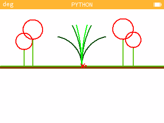
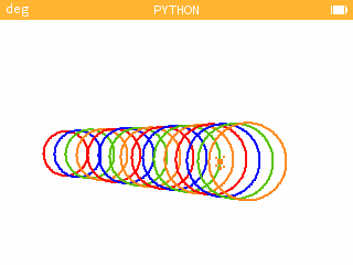
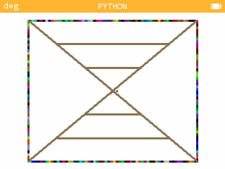
Nuwmorks Art with Turtle

Nuwmorks Art with Turtle


Announcement:   Twelve Days of Integrals starting on December 25, 2021.   Now on to the Python art!

Each picture will have the Nuwmorks script page where the code is located. 


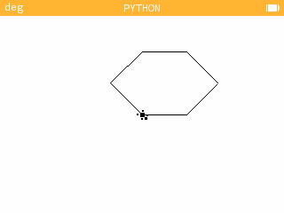
Hexagon


Download code:  

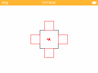
Square on Squares


Download code: 

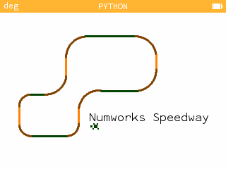
Numworks Speedway


Download Code:  

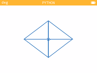
Four-Triangle Crystal


Download Code:


Turtle's Day Off


Download Code:


Looping Circles


Download Code:


Frame


Download Code:


Eddie

All original content copyright, © 2011-2021.  Edward Shore.   Unauthorized use and/or unauthorized distribution for commercial purposes without express and written permission from the author is strictly prohibited.  This blog entry may be distributed for noncommercial purposes, provided that full credit is given to the author. 

Saturday, December 18, 2021

Casio fx-CP400: Complex Numbered Graphs Using 3D Parametric Graphing Part II

Casio fx-CP400: Complex Numbered Graphs Using 3D Parametric Graphing Part II


Introduction


Note:  The procedure listed on today's post also applies to the Casio fx-CG 50 and fx-CG 500.  Since this involves the 3D Parametric Graphing mode, I don't think it will work on the ClassPad 300 or 330.


Here is a way to display complex-number functions: the use of 3D parametric graphing.   The general form will be:


x(s, t) = real(f(w)),   the real part of f(w)

y(s, t) = imag(f(w)),  the imaginary part of f(w)

z(s, t) = 0


where w = s + t*i,  i = √-1


The view window was set to:


angle Θ: -09

angle Φ: 0


Please keep in mind, the graph displayed will be the results, or the range, of f(w);


(s + t*i) ->  (x + y*i) = f(s + t*i)


To see s and t, execute Trace mode.  Read x and y for the real and imaginary part of the result.


For more details, please see last week's (12/11/2021) post.  


Examples


w = s + t*i,   x = real(f(w)), y = imag(f(w)), z = 0, Radians mode selected


Example 1:


f(w) = 2^w


x = 2^s * cos(t * ln 2)

y = 2^s * sin(t * ln 2)

z = 0


Example 2:


f(w) = w^(1/2) = e^(1/2 * ln w)


x = re((s + t*i)^0.5)

y = im((s + t*i)^0.5)

z = 0


Example 3:  


f(w) = w^3 + 1


x = s^3 - 3*s*t^2 + 1

y = -t^3 + 3*s^2*t

z = 0


Example 4:


f(w) = 2 * cos(w/2)


x = 2 * cos(s/2) * cosh(t/2)

y = -2 * sin(s/2) * sinh(t/2)

z = 0


Eddie 


All original content copyright, © 2011-2021.  Edward Shore.   Unauthorized use and/or unauthorized distribution for commercial purposes without express and written permission from the author is strictly prohibited.  This blog entry may be distributed for noncommercial purposes, provided that full credit is given to the author. 


Monday, December 13, 2021

Review and Instruction: Senario FC-500 Financial Calculator

Review and Instruction: Senario FC-500 Financial Calculator


Announcement:  Twelve Days of Integrals


In spirit of the Twelve Days of Christmas, I present the Twelve Days of Integrals:  starting December 25, 2021 to January 5, 2022.  I hope everyone has a happy, health, and sane holiday season!


Now on to the review.


Review: Senario FC-500 Financial Calculator


Quick Facts


Model: FC-500

Company: Senario

Years: ??, sometime in the 2010s?

Memory Register:  1 user memory with separate registers

Battery:  Battery, 2 x LR44

Screen:  12 digits

Logic:  Chain


I purchased the Senario FC-500 on eBay for relatively cheap.  The one I purchased did not come with an instruction manual, and I couldn't find one online.   


Through playing with the calculator and research with other financial calculators, the FC-500 models itself after the Hewlett Packard HP 12C.  


What makes this financial calculator a little unique is the wonderful presence of 40 U.S.-metric conversions.   The FC-500 is a feature rich financial calculator.  


I have yet to find instruction on how to change the number of decimal points displayed, if that is even available.  Most financial calculators default to the 2 decimal point setting, and that would be the expected setting.  This would be one of my sticky points for the FC-500, the other would be lack of user memory registers.  


The cash flow convention is followed:  positive for cash inflows (deposits and receipts), negative for cash outflows (payments).  The key with a magnifying glass over a document, which is located on the second row, sixth key (right-most key) is the compute/calculate key.  On this blog I will designate this key as the [(search)] button.


Features


*  Time Value of Money

*  Depreciation (Straight Line, Sum of the Years Digit, Declining Balance)

*  Sell/Cost/Margin (SEL, CST, MGN)

*  Interest Conversion:   Effective vs Nominal (APR)

*  Percent Calculations (%, percent change, % of total)

*  Currency conversions

*  Tax calculation (TAX+ and TAX-) 

*  Days between dates and date calculations (four digit years)

*  Statistics including Linear Regression


The rest will be an instruction sheet for those who are looking for a manual.  For anything I missed, you may want to look at the HP 10BII+ or HP 12C manual and it may fill the rest of the gaps.   Hope this helps.


Operating the FC-500


Time Value of Money (TVM)


PV:  present value

n:  number of payments, ×12

i:  periodic interest rate, ÷12

PMT:  payment

FV:  future value

Magnifying glass, designated as [(search)]:   Solve/CPT

B/E:  Beginning/End Toggle


Cash flow convention is followed


Example:

PV:  0.00

n:  3 years 

i:  3.86% compounded monthly

payment:  $50.00 per month


0 [ PV ]

3 [SHIFT] (×12)

3.86 [SHIFT] (÷12)

50 [+/-] [ PMT ]

[(glass)] [ FV ] returns 1,905.11893693


Amortization Procedure


1.  Enter n, i, PV, and any balloon amount in FV.

2.  Compute PMT.

3.  Enter period 1 to n, second period, press [SHIFT] (AMORT)

4.  Accumulated Interest,  [ X←→Y ], Accumulated Principal

5.  [ RCL ] [ PV ]: remaining balance

6.  [ RCL ] [ n ]: number of payments amortized

7.  To do the next batch, press [ SHIFT ] (AMORT), repeat steps 4 through 6


Example:

Loan:  $189,000.00

I/YR:  4.8% compounded monthly

Years: 20 years of monthly payments

No balloon payment

Amortize the first 2 years of 12 month payments


189000 [ PV ]

20 [SHIFT] [ ×12 ]

4.8 [SHIFT] [ ÷12 ]

0 [ FV ]

[(search)] [ PMT ] returns -1,226.529641804


First 12 Payments

0 [ n ] 12 [SHIFT] (AMORT)

Accumulated Interest:  -8,946.10891465

Accumulated Principal: [ X←→Y ], -5,772.24650183

Balance:  [ RCL ] [ PV ],  183,227.753498


Second 12 Payments

12 [SHIFT] (AMORT)

Accumulated Interest:  -8,662.86358088

Accumulated Principal: [ X←→Y ], -6,055.4918356

Balance:  [ RCL ] [ PV ],  177,172.261662


EFF/NOM conversion


Convert from NOM (APR) to EFF

payments per year [ n ]

nominal rate [ NOM ] 

[(search)] [ EFF ] 


Example:  NOM = 6%, payments per year = 24

24 [ n ]  6 [ NOM ]  [(search)] [ EFF ] returns 6.17570442629


Convert from EFF to NOM (APR)

payments per year [ n ]

nominal rate [ EFF ] 

[(search)] [ NOM ] 


Example:  NOM = 6%, payments per year = 24

24 [ n ]  6 [ EFF ]  [(search)] [ NOM ] returns 5.83397001049


Percent Change

old [ X←→Y ] new [ Δ% ]


Example:   4750 [ X←→Y ] 4200 [ Δ% ] returns -11.5789473684


Days Between Dates

first date [ X←→Y ] second date [SHIFT] (ΔDAYS)


Example:  3.141977 [ X←→Y ] 12.092021 [SHIFT] (ΔDAYS) returns 16,341

(M.DY year mode)

(March 14, 1977  to December 9, 2021)


Percent Total

whole [ X←→Y ] part [ %T ]


Example:  85 [ X←→Y ] 41 [ %T ] returns 48.2352941176


Date Addition

date [ X←→Y ] number of days [SHIFT] (DATE)

Day number:  1:  Monday to 7: Sunday


Example:  Determine the date 90 days from November 15, 2021?  (M.DY year mode)

11.152021 [ X←→Y ] 90 [SHIFT] (DATE) returns 2.132022-7

(Sunday February 13, 2022)


Tax Addition and Subtraction (Sales Tax)


To set the tax rate:  rate [SHIFT] (RATE SET)

To add the tax rate:  [TAX+]:   x∙(1+rate/100)

To subtract the tax rate:  [TAX-]:  x/(1+rate/100)


Example:  Set rate at 9.5%

200 [TAX+] returns 219

150 [TAX-] returns 136.986301369


Unit Conversions 


40 conversions

Use the blue keys:

[ ← ]:  metric to US

[ → ]: US to metric


Statistics - Linear Regression


Date:  x [ X←→Y ] y [ Σ+ ]


Registers used:   (not used for other purposes)

[ RCL ] [ 1 ]: N

[ RCL ] [ 2 ]: Σx

[ RCL ] [ 3 ]: Σx^2

[ RCL ] [ 4 ]: Σy

[ RCL ] [ 5 ]: Σy^2

[ RCL ] [ 6 ]: Σxy


Depreciation


[ n ]:  life of the asset in years

[ PV ]:  cost

[ FV ]:  salvage value, if any

[ i ]:  rate (for declining balance only)


year # [ SHIFT ] ( SL ):  Straight Line Depreciation  (press [ X ←→ Y] for book value)

year # [ SHIFT ] ( SOYD ):  Sum of the Year's Digits Depreciation  (press [ X ←→ Y] for book value)

year # [ SHIFT ] ( SL ):  Declining Balance Depreciation  (press [ X ←→ Y] for book value)


Simple Interest


n:  number of days

i:  annual interest rate

PV:  principal amount

Enter 0 in PMT and FV

Press [SHIFT] (INT) for simple interest


Example:

Calculate the simple interest of a 30-day loan of $1,400.00.  The annual rate is 6.5%.

1400 [ PV ]

30 [ n ]

6.5 [ i ] 

0 [ PMT ], 0 [ FV ]

[SHIFT] (INT) returns -7.583333333333  (360-day year)

[ X ←→ Y] -7.7945205479 (365-day year)


Eddie


All original content copyright, © 2011-2021.  Edward Shore.   Unauthorized use and/or unauthorized distribution for commercial purposes without express and written permission from the author is strictly prohibited.  This blog entry may be distributed for noncommercial purposes, provided that full credit is given to the author. 


Sunday, December 12, 2021

Six Integrals from Calculus I: Substitution vs Integration by Parts

Six Integrals from Calculus I:  Substitution vs Integration by Parts


Even slight differences integrands can change the strategy.  Observe.


Substitution


For these three integrals, the substitution u = x^2 will serve well.


Observe:

u = x^2

du = 2 x dx

du / 2 = x dx


∫ x sin x^2 dx

= ∫ 1/2 sin u du

= -1/2 cos u + C

= -1/2 cos x^2 + C


∫ x cos x^2 dx

= ∫ 1/2 cos u du

= 1/2 sin u + C

= 1/2 sin x^2 + C


∫ x e^(x^2) dx

= ∫ 1/2 e^u du

= 1/2 e^u + C

= 1/2 e^(x^2) + C


Integration by Parts


General:   ∫ u dv = u v - ∫ v du,  v and u are functions (usually of x)


∫ x^2 sin x dx

u = x^2, dv = sin x dx;   du = 2 x dx, v = - cos x


= -x^2 cos x + ∫ 2 x cos x dx

u = 2 x, dv = -cos x dx;  du = 2 dx, v = -sin x


= -x^2 cos x + 2 x sin x - ∫ 2 sin x dx

= -x^2 cos x + 2 x sin x - ∫ 2 sin x dx


∫ x^2 cos x dx

u = x^2, dv = cos x dx;   du = 2 x dx, v = sin x


= x^2 sin x - ∫ 2 x sin x dx

u = 2 x, dv = sin x dx;  du = 2 dx, v = -cos x


= x^2 sin x + 2 x cos x - ∫ 2 cos x dx

= x^2 sin x + 2 x cos x - 2 sin x + C


∫ x^2 e^x dx

u = x^2, dv = e^x dx;  du = 2 x dx, v = e^x


= x^2 e^x - ∫2 x e^x dx

u = 2 x, dv = e^x dx;  du = 2 dx, v = e^x


= x^2 e^x - 2 x e^x + ∫2 e^x dx

= x^2 e^x - 2 x e^x + 2 e^x + C

= e^x (x^2 - 2 x + 2) + C


Bottom line, being good at integration, like everywhere else in math, will require practice, experience, and maybe later in life, some retraining.  


Students, best of luck in your studies, in class and in life.  


Eddie 


All original content copyright, © 2011-2021.  Edward Shore.   Unauthorized use and/or unauthorized distribution for commercial purposes without express and written permission from the author is strictly prohibited.  This blog entry may be distributed for noncommercial purposes, provided that full credit is given to the author. 


Saturday, December 11, 2021

Casio fx-CP400: Complex Numbered Graphs Using 3D Parametric Graphing

Casio fx-CP400: Complex Numbered Graphs Using 3D Parametric Graphing


Introduction


Note:  The procedure listed on today's post also applies to the Casio fx-CG 50 and fx-CG 500.  Since this involves the 3D Parametric Graphing mode, I don't think it will work on the ClassPad 300 or 330.


Here is a way to display complex-number functions: the use of 3D parametric graphing.   The general form will be:


x(s, t) = real(f(w)),   the real part of f(w)

y(s, t) = imag(f(w)),  the imaginary part of f(w)

z(s, t) = 0


where w = s + t*i,  i = √-1


Other computer programs, like Mathematica, uses t and r for variables for 3D parametric graphing.   Check the manual for details.


For the Classpad,  re is the real part function, and im in the imaginary part function.   In the following examples, f(w) can be algebraically simplified to separate the real and imaginary parts.   


I set the x grid and y grid to 50, which is the maximum amount of points allowed.  This allows for most detailed graphs possible.  I set the window to viewing the z axis from the top.  On the Classpad, this is done by either pressing the [ z ] button or setting the angle settings on the View Window to:


angle Θ: -09

angle Φ: 0


Please keep in mind, the graph displayed will be the results, or the range, of f(w);


(s + t*i) ->  (x + y*i) = f(s + t*i)


To see s and t, execute Trace mode.  Read x and y for the real and imaginary part of the result.

I am using the Classpad, fx-CP400, because of the large screen which allows us to show the equations and the graph on one screen comfortably.  On each graph, I put f(w) as a text string on the graph screen.  For format, I set the line color to blue, green, or red (or any of the available colors) and I set the area to Clear (eraser icon).  

Examples


w = s + t*i,   x = real(f(w)), y = imag(f(w)), z = 0, Radians mode selected


Example 1:


f(w) = (w - i)^2 


x = s^2 - (t - 1)^2

y = 2 * s * (t - 1)

z = 0


Example 2:


f(w) = e^w


x = e^s * cos t

y = e^s * sin t

z = 0


Example 3:  


f(w) = 1/w


x = s / (s^2 + t^2)

y = -t / (s^2 + t^2)

z = 0


Example 4:


f(w) = sin w


x = sin s * cosh t

y = cos s * sinh t

z = 0


Really cool to see.  


Eddie 


All original content copyright, © 2011-2021.  Edward Shore.   Unauthorized use and/or unauthorized distribution for commercial purposes without express and written permission from the author is strictly prohibited.  This blog entry may be distributed for noncommercial purposes, provided that full credit is given to the author. 


Monday, December 6, 2021

Review: Sharp EL-344RB

Review: Sharp EL-344RB


Quick Facts


Model: Elsi Mate EL-344R

Company: Sharp

Years: production began around 2015

Memory Register:  1 independent memory

Power:  Solar with with LR1130 backup battery

Screen:  LCD, 10 digits

Logic:  Chain


First, the Basics


The EL-344R is a basic four-function calculator including percent and square root.   The memory keys [ M+ ] and [ M- ] not only complete the calculation but execute the appropriate storage arithmetic function.  The [ R∙CM ] key acts the dual function recall/clear memory.


Fractions and Approximations


You can enter fractions by using the [ a-b/c ] key.   There is a two digit limit to the numerator and denominator.  


Results can be converted to fractions.  However, the denominators offered are limited to n/2, n/4, n/8, n/16, and n/32.   If an exact fraction cannot be found, an APP indicator will show with an up or down arrow to show if the result has been rounded up or down.   In any case, the exact decimal is kept for future calculations.


Conversions


The large feature for the EL-344R is the set of metric-U.S. conversions.   Conversions include (not an all-exhaustive list):


*  temperature (°F/°C)

*  length (in/cm, ft/m, yd/m mi/km)

*  area (in^2/cm^2, ft^2/m^2, yd^2/m^2, acre/ha etc.)

*  volume (in^3/cm^3, ft^3/m^3, US gal/L, etc.)

*  weight (oz/g)


There are 44 preset conversions.    You can use the [ >A ] and [ <B ] keys allow you to set a custom conversion rate and use it for conversion calculations.


The conversions are nice, quick, and easy, and gives regular calculator an extra useful feature.   


Verdict


I like the rich set that compliments the EL-344R.   To me, the selling point is the nice set of conversions.   The keys are easy to press and I love the clear screen with large digits.  Recommended.


Eddie


All original content copyright, © 2011-2021.  Edward Shore.   Unauthorized use and/or unauthorized distribution for commercial purposes without express and written permission from the author is strictly prohibited.  This blog entry may be distributed for noncommercial purposes, provided that full credit is given to the author. 


Sunday, December 5, 2021

HP 17B and HP 27S: Using the Solver for Recursive Functions

HP 17B and HP 27S: Using the Solver for Recursive Functions


Introduction


A simple store and recall procedure can be used with the solver.   


One Initial Condition


u_n = f(u_n-1) with the initial condition u_0


Let B = u_n and A = u_n-1, set up the solver as:


B = F(A)


Initial condition:

u_0 ( A ) ( B )


Subsequent calculations:

[ RCL ] ( B )* [ STO ] ( A ) ( B )


*RCL B is not necessary if you go straight to the next calculation.  


Example:   

u_n = 4*u_n-1 - 3, u_0 = 3


Setup:  B=4×A-3


3 ( A ) ( B )

Result:  9


[ RCL ] ( B) [ STO ] ( A ) ( B )

Result:  33


[ RCL ] ( B) [ STO ] ( A ) ( B )

Result:  129


[ RCL ] ( B) [ STO ] ( A ) ( B )

Result:  513


Two Initial Conditions


u_n = f(u_n-1, u_n-2) with the initial conditions u_0 and u_1


Let C = u_n, B = u_n-1, and A = u_n-2 and set up the solver as:


C = F(A, B)


Initial condition:

u_0 ( A ) u_1 ( B )  ( C )


Subsequent calculations:

[ RCL ] ( B )* [ STO ] ( A ) ( B )


Example:


The Fibonacci Sequence:

u_n = u_n-1 + u_n-2; with u_0 = 1, u_1 = 1


Setup:  C=B+A


1 ( A ) 1 ( B ) ( C )

Result: 2


[ RCL ] ( B ) [ RCL ] ( A ) ( C )

Result:  3


[ RCL ] ( B ) [ RCL ] ( A ) ( C )

Result:  5


[ RCL ] ( B ) [ RCL ] ( A ) ( C )

Result:  8


Nothing to it.


Eddie 


All original content copyright, © 2011-2021.  Edward Shore.   Unauthorized use and/or unauthorized distribution for commercial purposes without express and written permission from the author is strictly prohibited.  This blog entry may be distributed for noncommercial purposes, provided that full credit is given to the author. 


Saturday, December 4, 2021

HP 17B and HP 27S: Derivatives to the Nth Order (and TI-84 Plus CE Python 5.7 update)

 HP 17B and HP 27S: Derivatives to the Nth Order


With the Solver of the HP 17B family, HP 27S, and the HP 19B calculator, we can calculate derivatives of any order.  Four derivatives are presented here.  You can use any name you want other than those presented here.  Each derivative is to the kth order. 


Derivative 1:   d^k/dx^k a × x^n 


N and K must be positive integers, D is the value of the derivative  


DER1: D=A×X^(N-K)×PERM(N:K)


Example:

Input:  N = 2, K = 1, A = 3, X = 1.5

Result:  D = 9


Derivative 2:   d^k/dx^k e^(a × x) 


K must be a positive integer, D is the value of the derivative


DER2: D=A^K×EXP(A×X)


Example:

Input:  A = 1.8, K =3, X = 3

Result:  D = 213.4409


Derivatives 3 and 4 will require trigonometric functions, which are not available on the HP 17B family.   It is recommended you set the calculator to Radian angle mode.


Derivative 3:  d^k/dx^k sin(a × x)


DER3: D=IF(MOD(K:2)=0:(-1)^(K÷2)×A^K×SIN(A×X):(-1)^((K+3)÷2)×A^K×COS(A×X))


Examples:

Input:  A = 0.75, X = 0.66, K = 2

Result: D = -0.2672


Input:  A = 0.75, X = 0.66, K = 3

Result: D = -0.3712


Derivative 4:  d^k/dx^k cos(a × x)


DER4: D=IF(MOD(K:2)=0:(-1)^(K÷2)×A^K×COS(A×X):(-1)^(K÷2+1÷2)×A^K×SIN(A×X))


Examples:

Input:  A = 0.75, X = 0.66, K = 2

Result: D = -0.4950


Input:  A = 0.75, X = 0.66, K = 3

Result: D = 0.2004


Eddie


All original content copyright, © 2011-2021.  Edward Shore.   Unauthorized use and/or unauthorized distribution for commercial purposes without express and written permission from the author is strictly prohibited.  This blog entry may be distributed for noncommercial purposes, provided that full credit is given to the author. 


  Casio fx-7000G vs Casio fx-CG 50: A Comparison of Generating Statistical Graphs Today’s blog entry is a comparison of how a hist...