Friday, September 25, 2015

HP Prime Spreadsheet App Tutorial 9: Custom Functions in the Spreadsheet App and the AMORT Function

HP Prime Spreadsheet App Tutorial 9:  Custom Functions in the Spreadsheet App and the AMORT Function


Lesson 9 Objectives:

* Defining a Custom Function
* Using a Custom Function in the Spreadsheet
* Using the AMORT Function

Background:

The AMORT function is found by pressing [ Menu ], 6.   It’s syntax is:

AMORT(range where you want your output, number of periods, annual interest rate, present value, payment, [payments per year (default is 12), grouping (default is 12), Beg (FALSE for end of period, TRUE for beginning of period payments), fix (default is 2)], [“Configuration”])

Anything enclosed in brackets [ ] are optional arguments.  I recommend that you type a single cell for the range of output, letting the Spreadsheet app worry about calculating the appropriate size of the amortization table.

Steps:

Setup:

1.     Clear the Spreadsheet.
2.    Select the cell with the hp logo.   Set the spreadsheet to Fixed format with 2 decimal places by using the (Format) command.

Create the Function:

3.     Press the [ Home ] key, then press [ Shift ], [x t θ n] (Define).  This takes you to the Define screen.  You will see two fields: Name and Function.  The order of the arguments take is taken from when they first appear in the Function.
4.    Name the function PYMT for payment.
5.    Type the formula in the Function field:  (-.01*R/C*P) / (1 – (1+.01*R/C)^-N).  Once you check it for accuracy, press (OK).
6.    You can test the function PYMT on the Home Screen.  PYMT(R,C,P,N) has four arguments:
·         R = annual interest rate
·         C = number of payments per year
·         P = present value
·         N = number of periods


Back to the Spreadsheet:

7.     Type the following labels:
·         A1 = “N”
·         B1 = “INT”
·         C1 = “PV”
·         D1 = “PMT”
8.    Type the following amounts and formulas:
·         A2 = 360  (for 360 payments)
·         B2 = 5  (for an annual interest rate of 5%)
·         C2 = 140000  (for the present rate of $140,000)
·         D2 = PYMT(B2,12,C2,A2)  (to calculate the payment, which should be -751.55)
9.    Go to cell A4.  Type =AMORT(A4,A2,B2,C2,D2,12)*.  An amortization chart is produced.

* There was an error pointed to me by Michael Kokot.  It is corrected now.  I thank you Kokot for bringing it to my attention.

Eddie 10/8/2015


This concludes Lesson 9.  Hope you find this helpful,

Eddie


This blog is property of Edward Shore, 2015.


HP Prime Spreadsheet App Tutorial 8: Statistical Analysis

HP Prime Spreadsheet App Tutorial 8:  Statistical Analysis

 Lesson 8 Objectives:

* Use One Variable Statistical Analysis and Customize its format
* Calculation regression analysis


Part 1:  One Variable Statistics


How to find STAT1:  In the Spreadsheet, press [ Menu ], 7.

Simple Syntax:
STAT1(range of data, “configuration”)

STAT1 can be expanded for more uses, please consult the HP Prime Graphing Calculator User Guide for details (pg. 345-346).  There is also a two-variable version, STAT2. 

Configuration is a string and is optional.  This allows us to refine or select just what we want to see.  Each symbol is separated by a single space.  

STAT1 configuration
Common symbols to use:
Symbol
Function
How to Get it
h
Place row labels
Insert h (lower case) at the beginning at the configuration string.  “h “
H
Place column labels
Insert H (upper case) at the beginning at the configuration string.  “H “
Mean
Type “+CHAR(57344)+”
s
Standard Deviation
Type “s “
σ
Population Deviation
Get σ from [Shift], [ 6 ] menu
Σ
Sum
Get Σ from [Shift], [ 6 ] menu
2
Square Symbol, add to s, σ, or Σ
Attach “+CHAR(178)+”
n
Number of data points
Type “n”

Please see the steps for an example.

Note:  I had the calculator set to Fix 3. 

Part 1 Steps:

1.     Enter the following data:
·         A1 = 5.250
·         A2 = 5.990
·         A3 = 6.345
·         A4 = 6.989
·         A5 = 7.210
·         A6 = 7.116
·         A7 = 7.385
2.    Go to cell B1.  Enter =STAT1(A1:A7).  You will see all the possible results and the labels.  The next steps will show you how to use specific configuration.
3.    Select cells B1:C16 and press the [  Del ] key.  We have to manually clear the results.  The next step will detail how to display only the number of data points (n), mean (x̅), and standard deviation (s).
4.    Again, go to B1 and enter =STAT1(A1:A7, “n x̅ s”). 
·         Keystrokes:  [Shift], [ . ] (=), [Menu], 7 for STAT1, [ ( ) ], type A1:A7, [ , ], [Shift], [ 0 ] ( “ “ ), [ALPHA], [Shift], [ ( ) ] (n), [SPACE], [ → ], [ + ], type CHAR(57344), [ + ], [Shift], [ 0 ] ( “ “ ), [ALPHA], [Shift], [ 9 ] ( s ), (OK)
·         Note that you will see only numeric results.   If you want labels, we will need to add an h (for Row Headers) or H (for Column headers) to the beginning of the configuration.
5.    Edit B1 to read =STAT1(A1:A7, “h n x̅ s”).  You should see row headers as well as the wanted results.


Part 2:  Regression Analysis


Simple Syntax:
REGRS(range, model number)

Please refer to the HP Prime User Guide, pg. 347 for all the details of this command.

Common regression models and the number that represents them:

1 for Linear.  (y = m*x + b)
2 for Logarithmic (y = m*ln x + b)
3 for Exponential (y = b*e^(m*x))
4 for Power (y = b*x^m)
6 for Inverse (y = m/x + b)
9 for Quadratic (y = a + b*x + c^2)

Part 2 Steps:

6.     Reset the Spreadsheet.
7.    Enter the following labels and data:
·         A1 = “Hours”
·         B1 = “Sales”
·         C1 = “Data”
·         A2 = 50, B2 = 4300
·         A3 = 52, B3 = 4800
·         A4 = 51, B4 = 4600
·         A5 = 49, B5 = 4480
·         A6 = 48, B6 = 4270
·         A7 = 50, B7 = 4330
8.    Go to cell C2.  Type =REGRS(A2:B7, 1).  This performs linear regression on the data.

Note:  You can add a custom configuration to REGRS.  See the manual for details. 


That is it for Lesson 8.  In Lesson 9, we’ll cover using custom functions in the Spreadsheet app.  Until next time,

Eddie


This blog is property of Edward Shore, 2015.   Post 501!

HP Prime Spreadsheet App Tutorial 7: Absolute References


HP Prime Spreadsheet App Tutorial 7:  Absolute References


Lesson 7 Objectives:

* Use Absolute References

Background:

When a formula is copied into different cells, the Spreadsheet app adjust the cells used.  For example, say that cells A1:B10 have numeric data and I want to find the sum of each column.  I type =SUM(A1:A10) in cell A11.   I don’t have to readjust the formula if I just copy the formula from cell A11 to B11.  The app automatically adjusts the formula in cell B11 to =SUM(B1:B11).  This is known as relative reference.

This is a great feature but there times where we don’t want the cell reference to change.  Say in cell C1 I have a rate that is multiplied to the sum of both columns.  In this case, we can use an absolute cell reference, so that when the formula is copied from A11 to B11, the C1 reference remains locked.  To make an absolute reference, add a dollar sign ($) to the column and row indicators.  Hence, in our example, A11 would contain the formula =$C$1*SUM(A1:A10).  When the formula is copied to B11, its formula would have =$C$1*SUM(B1:B10).

We can freeze only the column ($C1), only the row (C$1), or both ($C$1).

In today’s lesson, we are going to build a spreadsheet that contains item and the tax for each item (see picture at the top of this blog entry).

Steps:

1.     Select the cell with the hp logo (upper left hand cell).  Format the spreadsheet so that it is set to 2 decimal places.   (Format), 1 for Number Format, 3 for Fixed.  (Format), 1 for Number Format, 8 for Decimal Places, select 2.
2.    Enter the text in the following cells:
·         A1:  “Rate”
·         B2:  “Price”
·         C2:  “Tax”
·         A3:  “Discs”
·         A4:  “Paper”
·         A5:  “Staples”
·         A6:  “USB”
3.    Enter the following amounts:
·         B1 = 0.09   (9%)
·         B3 = 9.99
·         B4 = 8.99
·         B5 = 14.99
·         B6 = 12.99
4.    Go to cell C3.  Press (Select) and then arrow down to C6.  The range C3:C6 should be selected.
5.    Type =B3*$B$1.  B1 will be an absolute reference.  You can get the $ sign by pressing the soft key ( $ ) while you are entering a formula, text, or numeric data.
6.    Change the rate in cell B1 (use the decimal format).  Observer the change in cells C3:C6.


This concludes Lesson 7.  On the next installment we will work with statistical analysis.  Until next time,

Eddie


Note:  This is my 500th post on this blog.  Thank you to you all!


This blog is property of Edward Shore, 2015.


HP Prime Spreadsheet App Tutorial 6: Row and Column References in Formulas

HP Prime Spreadsheet App Tutorial 6:  Row and Column References in Formulas


Lesson 6 Objectives:

* Use Row and Col in spreadsheet formulas

We can use formulas that are determined where the cell position.  Use Row for row references and Col for column references.  Be aware that Row and Col are case-sensitive.  

What value Row takes is almost obvious since rows are labeled numerically.  Columns are labeled alphabetically.  The values each column assign is:

1 for column A,
2 for column B,
3 for column C,
4 for column D,
5 for column E, and so on.

Part 1:  Build a Spreadsheet of Fibonacci Numbers with the first column of row numbers.


1.     Start by clearing the spreadsheet ( [ Shift ], [ Esc ] (Clear), (OK) ).
2.    Select the header cell for Column A.  The header cell is above cell A1.  Enter the formula =Row.
3.    Select the header cell for Column B, above B1.  Type the following formula:
=( ((1 + √5)/2)^Row – ((1 - √5)/2)^Row ) / √5


Part 2:  Build a Spreadsheet of Powers


4.     Clear the Spreadsheet.
5.    Select the upper left hand cell, with the hp logo.
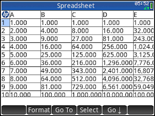
6.    Type =Row^Col.


That concludes Lesson 6.  Next we will tackle using absolute references.  Have a great day,

Eddie


This blog is property of Edward Shore,  2015.

Sunday, September 20, 2015

HP Prime Spreadsheet App Tutorial 5: Spreadsheets and Histograms

HP Prime Spreadsheet App Tutorial 5:  Spreadsheets and Histograms


Lesson 5 Objectives:

* Generate a random list of integers for a column
* Store a Spreadsheet column to a Statistics Variable
* Use a Spreadsheet column in a histogram

Generate a random list of integers:

RANDINT(length of list, lower limit, upper limit).  The result is a list.


Steps:

1.     Start by selecting the header cell for Column A.  Press [ Toolbox ], 5 for Probability, 4 for Random, 2 for Integer to call the RANDINT function.   A list a generated, so no equals sign is needed.  Enter 100 for the length of list, 0 for the lower limit, and 100 for the upper limit.  The result is RANDINT(100,0,100).  Press the soft key ( OK ).
2.    Name Column A DATA.   Go to the header cell, enter DATA, and press on the soft key ( Name ).
3.    Press the [ Home ] button.  Select the D1 variable from the Statistics 1Var app by pressing [ Vars ], the ( App ) soft key, then Statistics 1Var, then Numeric, and D1. 
4.    Continue by entering DATA.   (colon, equals, DATA).   The complete command should be Statistics_1Var.D1DATA.
5.    On to the Histogram:  Press the [ Apps ] and choose the Statistics 1Var app.   You’ll be taken to the Num view and D1 should be filled in.
6.    Press the [ Symb ] key for the Symbolic view.   Enter D1 for H1 and select Histogram. 
7.    Press [ Shift ], [ Plot ] (Plot Setup).   Change the H Width to 10. 
8.    Press [ View ] and select Autoscale.    This Histogram is complete.


This concludes Lesson 5.  I plan to post additional lessons in the near future.   

Eddie


This blog is property of Edward Shore,  2015.

HP Prime Spreadsheet App Tutorial 4: Naming Columns and Using them Outside of Num View


HP Prime Spreadsheet App Tutorial 4:  Naming Columns and Using them Outside of Num View


Lesson 4 Objectives:

*  Name Columns
*  Use Columns in formulas
*  Use Named Columns outside the Spreadsheet

Note:  I had the calculator set to Fix 3 as the number format. 

Steps:

1.    Start with a clear spreadsheet.  To recall, to reset the spreadsheet, press [ Shift ], [ Esc ] (Clear) and confirm at the prompt.
2.    Type 10, 20, 30 and 40 in cells A1, A2, A3, and A4, respectively.
3.    Select the header cell of column A, which is above the cell A1. 
4.    Name a Column:  type COL1.  To give the column that name, touch the soft key ( Name ).  You won’t need quotes to name columns. 
5.    Let’s name Column B.   Select the header cell for column B.  Type COL2 and touch the soft key ( Name ).
6.    Enter a Formula Spanning Multiple Cells:  In column B, let’s double all the values in column A.   Start at cell B1, and select cells B1 through B4 by use the ( Select ) soft key.  Enter =A1*2.  Note how the formula fills down to B4 and uses the appropriate cell. 
7.    Recalling Columns Outside of the Spreadsheet:  Press the [ Home ] key and recall COL1 and COL2.  You can do this by typing the names or recalling them from the Vars-Spreadsheet-Cells menu.

Caution:  Only columns, rows, and individual cells can be named.  Matrix-like ranges, such as A1:B2 cannot be named.


In Lesson 5, we’re taking a spreadsheet column to the Statistics 1Var app.   See you next time,

Eddie


This blog is property of Edward Shore, 2015.


HP Prime Spreadsheet App Tutorial 3: Adding Labels, Entering Numeric Calculations, Changing Numeric Format of Cells, and Extending Columns

HP Prime Spreadsheet App Tutorial 3:  Adding Labels, Entering Numeric Calculations, Changing Numeric Format of Cells, and Extending Columns


Lesson 3 Objectives:

* Adding Labels to Cells
* Entering Numeric Calculations
* Changing the Numeric Format of Cells
* Expanding the Length of a Column

Note:  I had the calculator set to Fix 3 as the number format. 

Objective:
A calculator company wants to find out the profit of their graphing calculator sales for a week from a local store.  The store sells the calculator for $149, including tax.  It costs the company $69 per calculator for manufacturing and research costs, plus an estimated fixed cost of $2,500.  For the week in question, 150 calculators were sold.  Find the profit.

Steps:

1.    We’ll start with the labels Sales, Costs, and Profit.  Use cells A1, A2, and A3, respectively.  Enter labels as strings.  So, for A1, enter “Sales”; “Costs” for A2; and “Profit” for A3.
2.    The next step is to add the numerical calculations.  We are going to have the HP Prime execute the numeric calculation.  For sales, enter =150*149.   Put the calculation in cell C1.
3.    For C2, calculate the costs.  The formula is =150*69+2500.
4.    For C3, calculate the profit.   Enter =C1-C2.  The result should be $9,500.00.
5.    Change the format of the cells containing numbers to show 2 decimal numbers.   To do this, first select C1.  
6.    Next press the (Select) soft key.   It turns into the soft key (Sel *)  (The * represents a solid circle.  You are in Select Mode.  Any cell you go to using the arrow keys selects that cell.  In this case, press down [ ↓ ] twice to select cells C2 and C3.
7.    Choose the Fixed Format:  Press the (Format) soft key and select 1 for Number Format, then 3 for Fixed.  
8.    Choose 2 Decimal Places:  Press the (Format) soft key and select 1 for Number Format, then 8 for Decimal Places, then 2.
9.    Select the Header Cell of Column C:  Select the header cell of column C, which is above cell C1.  You can tap the header cell or use the arrow keys.  Unfortunately the (Go To) feature won’t let you select header cells.
10.  Enlarge Column C:  Press the (Format) soft key and select 8 for Column ←→ .   Enter 125.  Column sizes are measured in pixels and not in font size.


Next time, we will name columns, use names in a formula, and recall columns in places outside the Spreadsheet App Num View.

Have a great day, 
Eddie


This blog is property of Edward Shore, 2015.

Spotlight: Akron Brass FireCalc Pocket Computer

Spotlight: Akron Brass FireCalc Pocket Computer Welcome to a special Monday Edition of Eddie’s Math and Calculator blog. Thi...