Eddie's Math and Calculator Blog: July 2018

Friday, July 27, 2018

HP Prime: 3D Graphs July 2018 Gallery

HP Prime: 3D Graphs July 2018 Gallery

All graphs are made with the initial rangers x = [-4, 4], y = [-4, 4], and z = [-4, 4] rotated at different angles. The function variable for 3D graphs for the HP Prime is FZ# (# is 0-9).

z = cos (xy) * cos(2xy) * cos(3xy)

z = e^(-sin(2xy)*cos(xy)/2)

z = cos y * (e^(-x^2/2) – e^(x^2/8))

z = sin(x*y) * cos(x*y) + sin(x*y)^2 * cos(x*y)

z = x^4 * y * cos(x*y) * e^(x*y)

z = ± √(x^2 – y^2)

z = ± |sin(x*y) – cos(x*y) + x* e^y|

z = y^2 * sin x * Γ(x/6)

z = x * sin(|x^2 + y^2|)

Until next time, have a great weekend and see in you August!

Eddie

All original content copyright, © 2011-2018. Edward Shore. Unauthorized use and/or unauthorized distribution for commercial purposes without express and written permission from the author is strictly prohibited. This blog entry may be distributed for noncommercial purposes, provided that full credit is given to the author. Please contact the author if you have questions.

Wednesday, July 25, 2018

HP Prime: Firmware Update (13865, date 2018.07.06)

HP Prime: Firmware Update (13865, date 2018.07.06)

There is a new update to the HP Prime firmware. The new version is 13865.

You can find the file and details here:

Details and file:

http://www.hpmuseum.org/forum/thread-11097.html

http://www.hpmuseum.org/forum/thread-11092.html

Firmware download: ftp://ftp.hp.com/pub/calculators/Prime/

I haven’t had much chance to work with the new firmware, however according to the release information, some of the highlights are:

* There is a new red indicator when the HP Prime’s power reaches below 10%.

* All integrals in HOME mode will calculate numerical results. Previously results are returned in either numerical or exact answers. Exact answers will still be provided in CAS mode.

* You can control the amount of time until the HP Prime dims its screen. The screen is dimmed when you do nothing on the calculator after a set amount of time. The time is set in milliseconds as a base integer (30,000 in decimal or 7530_16 in hexadecimal). The variable is TDim found in the Vars-Setting menu.

* The command EVAL is said to now help INPUT with local variables. I haven’t played around with this yet.

* Updated CAS and improvements

As a note, there the HP Prime now gets a new processor G2. To find out what hardware version you have, press [Help], press the soft key (Tree), scroll up, select About HP Prime. I have hardware revision C. The threads on the MoHPC site goes into more details. The reason why I mention this is if you have trouble updating your HP Prime, the firmware files may need to be in a new folder. The folder is:

Hardware C (and I’m assuming this will work for A):

(your drive) \HP Connectivity Kit\Firmware\PrimeG1

Thank you to HP and HP Museum of Calculators!

Happy Computing,

Eddie

Monday, July 23, 2018

Algebra: Multiplying a * b Trick (Using the Difference between a and b)

Algebra: Multiplying a * b Trick (Using the Difference between a and b)

Can we find a formula to find products where two values are an equal-distant apart

The Values of a and b Differ by 2

Let a and b be real numbers which differ by 2, that is b – a = 2. Here I am assuming that b > a.

Let n be the midpoint between a and b. That is:

n = b – 1 and

n = a + 1

Therefore:

b = n + 1

a = n - 1

Then:

a * b

= (n - 1) * (n + 1)

= n^2 - n + n – 1

= n^2 - 1

Example: 51 * 49

Notice that:

51 – 49 = 2, and

51 - 1 = 50

49 + 1 = 50

Hence:

51 * 49 = 50^2 – 1 = 2499

Can we expand this included products of a * b, where the difference is b – a = 2 * w

The Values of a and b Differ by 2*w

Let’s look at a more general case.

Let b – a = 2*w

Then:

b = n + w and a = n – w

Then:

a * b

= (n – w) * (n + w)

= n^2 – n*w + n*w – w^2

= n^2 – w^2

Example: 37 * 43.

43 – 37 = 6

w = 6/2 = 3

Then:

n = 43 – 3 = 37 + 3 = 40

Then:

37 * 43 = 40^2 – 3^2 = 1600 – 9 = 1591

Try another example: 57 * 49

57 – 49 = 8

8 / 2 = 4

57 – 4 = 53, 49 + 4 = 53

Then:

57 * 49 = 53^2 – 4^2 = 2809 – 16 = 2793

In summary for a * b with b > a.

Let w = (b – a)/2 and n = a + w or n = b – w

Then a * b = n^2 – w^2

Eddie

Wednesday, July 18, 2018

Fun with the FX-603P Emulator

Fun with the FX-603P Emulator

Author for the Emulator: Martin Krischik

Link to Emulator (Android): https://play.google.com/store/apps/details?id=net.sourceforge.uiq3.fx603p&hl=en

Web Page: http://fx-602p.krischik.com/index.php/FX-603P/HomePage

Cost: $5.99 (there is an fx-602P scientific calculator emulator for $4.99, similar programming language but only 10 programming spaces instead of 20)

The app is emulates the 1990 Casio fx-603P calculator.

Decibels to Pressure

Program: (29 steps)

“DB?” HLT ÷ 20 = 10^x * 2E-5 = “Pressure:” HLT

Examples:

DB = 30 dB; Result: 6.32455532 * 10^-4 N/m^2

DB = 120 dB; Result: 20 N/m^2

Turn Performance

Given a plane’s true air speed (TAS in knots), stall speed (in knots), and required bank turn (in degrees), the following are calculated:

1. G force

2. Normal stall speed for the plane during the turn (knots)

3. Turn diameter (nautical miles)

4. Time it takes for the turn to be complete (in minutes)

Formulas:

G = 1/(cos(bank))

Stall speed = normal stall speed * √G

Diameter = TAS^2 / (34208 * tan(bank))

Time = (0.0055 * TAS) / tan(bank)

Memory Registers:

Input:

M00 = TAS, M01 = Stall speed, M02 = Bank

Output:

M03 = G force, M04 = resulting stall speed, M05 = diameter, M06 = time

Program: (110 steps)

DEG “TAS?” HLT Min00

“Norm. Stall?” HLT Min01

“Bank?” HLT Min02

MR02 cos 1/x Min03 “G:” HLT

MR03 √ * MR01 = “Stall Speed:” HLT

MR00 x^2 ÷ ( MR02 tan * 34208 ) = Min05 “Diameter:” HLT

0.0055 * MR00 ÷ MR02 tan “Time:” HLT Min06

Notes:

DEG: [ MODE ] [ 4 ]

Example:

Inputs:

TAS: 123 knots

Norm. Stall: 60 knots

Bank: 44.8°

Results:

G: 1.409302674

Stall Speed: 71.22843498 knots

Diameter: 0.445363387 n.m.

Time: 0.681239424 minutes (about 40.87 seconds)

Source: “Turn Performance” HP 65 Aviation Pac-1 Hewlett Packard. 1974

Sum of a Function

This program uses the subroutine (under P9 with the variable MinF, or any register M04 or after) to calculate the summation:

Σ f(x) for x = a to b

The sum is stored in M03.

Note: when entering a new f(x), clear P9 (MODE, 3, P9, AC) first before entering the new function. It’s a lot cleaner.

Main Program: (34 bytes)

0 Min03

“a?” HLT Min01

“b?” HLT Min02

MR02 – MR01 + 1 = Min00

Lbl0

MR01 GSBP9 M+03

1 M+01

DSZ Goto0

MR03 “Σ=”

Note:

Lbl0: [ LBL] [ 0 ]

GSBP9: [GSB] [ P9 ]

Goto0: [ GOTO ] [ 0 ]

The character Σ: (in ALPHA) [SHIFT] [ 7 ]

Memory F: [ Min ], [ MR ], etc. [EXE] for F.

Examples:

Σ n^2 + 3*n – 6 for n = 1 to 8

Subroutine:

Min0F x^2 + 3 * MR0F – 6 =

Result: 264

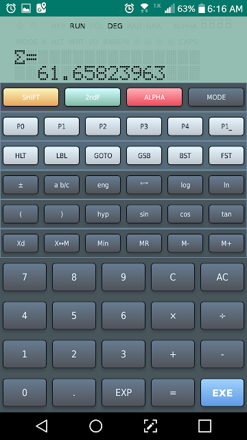
Σ (n^3 – 1)/(n^2 + 1) for n = 0 to 11

Subroutine:

( Min0F x^y 3 – 1 ) /div (MR0F x^2 + 1 ) =

Result: 61.6582396282

Combinations: where Repetition is allowed

The program calculates the number of combinations where repeats are allowed.

nHr = (n + r – 1)! / (r! * (n -1)!)

Program: (39 steps)

“n?” HLT Min01

“r?” HLT Min02

( MR01 + MR02 – 1) x!

÷ ( MR02 x! * ( MR01 – 1 ) x! )

= “nHr=”

Examples:

Input: n = 5, r = 3. Result: 35

Input: n = 12, r = 6. Result: 12376

Aviation: Rate of Climb

This program calculates the rate-of-climb (ft/min) when plane increases the elevation (in feet) given the distance to the mountain (in nautical miles, n.m.) and the true air speed (TAS, in knots).

Formula:

ROC = ( TAS * ΔALT ) / (60 * √(dist^2 + (ΔALT/6077.1155)^2) )

Program: (88 steps)

6077.1155 Min0F

“TAS (knots)?” HLT Min01

“CHG ALT (ft)?” HLT Min02

“DIST (n.m.)?” HLT Min03

( MR01 * MR02 ) ÷

( 60 * ( MR03 x^2 + (

MR02 ÷ MR0F ) x^2

) √ = “ROC:”

Example:

Input:

TAS = 87 knots

CHG ALT = 4800 ft

DIST = 13.3 n.m.

Result:

522.3878955 ft/min

Source: “Rate of Climb and Descent” HP 65 Aviation Pac-1 Hewlett Packard. 1974

Eddie

Thursday, July 12, 2018

Fun with the Radio Shack EC-4026

Fun with the Radio Shack EC-4026

(Equivalent of the Casio fx-4500P)

Programming Notes

The syntax for prompting for variables and displaying results are slightly different from the usual Casio programming language (as I mentioned, the EC-4026 is a clone of the fx-4500P). Check out the unusual If-Then-Else-End structure as well.

Prompting Syntax:

{var} : var “prompt string”

Example:

{X}: X”ENTER X”

Display Syntax:

Calculation

“Display string” ◢ (solid right triangle, [2ndF] [↑])

Example:

“F(X)=” ◢

The If-Then-Else-End Structure:

If condition ⇒ do if the condition is true ⇏do if condition is false ◺ (clear right triangle, [2ndF] [√])

Note: I symbolize the [x^y] by ^.

Finding the Monthly Payment of a Mortgage with Total Interest Paid and Total Cash Outflow

Program MORTGAGE:

L1 Fix 2

L2 {A}: A”LOAN AMOUNT”

L3 {Y}: Y”YEARS”

L4 {I}: I”RATE”

L5 I = I/1200

L6 N = Y*12

L7 P = A*(I(1+I)^N)/((1+I)^N-1)

L8 “MONTHLY PMT” ◢

L9 N*P

L10 “OUTFLOW” ◢

L11 N*P-A

L12 “TOTAL INTEREST” ◢

L13 Norm

Example:

A: Loan is $250,000.00

Y: 30 years

I: Interest rate of 4%

Results:

P: Payment: $1,193.59

Outflow: $429,673.77

Total Interest: $179,673.77

Midlength, Height, and Area of a Trapezoid

Program TRAPEZIOD:

L1 {A}

L2 {B}
L3 {C}

L4 {D}

L5 H = √((-A+B+C+D)*(A-B+C+D)*(A-B+C-D)*(A-B-C+D))/(2*Abs(B-A))

L6 M = (A+B)/2

L7 K = M*H

L8 M

L9 “MIDLENGTH” ◢

L10 H

L11 “HEIGHT” ◢

L12 K

L13 “AREA” ◢

Quadratic Equation A*x^2 + B*x + C = 0

Program QUAD:

L1 {A}: A”A”

L2 {B}: B”B”

L3 {C}: C”C”

L4 D = B^2-4*A*C

L5 D<0 ⇒ Goto 1 ◺

L6 X = (-B + √D)/(2A) ◢

L7 Y = (-B - √D)/(2A) ◢

L8 Goto 0

L9 Lbl 1

L10 X = -B/(2A)

L11 “REAL” ◢

L12 Y = √(Abs D)/(2A)

L13 “IMAG” ◢

L14 Lbl 0

L15 “DONE” ◢

Example:

3x^2 + 6x – 1 = 0; A = 3, B = 6, C = -1

Result: 0.154700538, -2.154700538

3x^2 + 6x + 10 = 0; A = 3, B = 6, C = 10

Result: REAL: -1, IMAG: 1.527525232. -1 ± 1.527525232i

Minimum Loss Matching

Variables:

Input: Y = Z0, Z = Z1

Output:

R = R1

S = R2

L = Loss Marching

Program MINLOSS:

L1 1: “Z1<Z0” ◢

L2 {Y}: Y”Z0”

L3 {Z}: Z”Z1”

L4 L = √(1 – Z/Y)

L5 R = Y*L: “R1”◢

L6 S = Z/L: “R2” ◢

L7 L = 20 log (√(Y/Z) + √(Y/Z – 1)): “LOSS” ◢

Example:

Input:

Y: Z0: 15

Z: Z1: 10

Output:

R1: 8.66025 Ω

R2: 17.32051 Ω

Loss: 5.71948

Add Two Polar Numbers

Polar and Rectangular conversions

Variable	Rectangular Results	Polar Results
V	x	r
W	y	θ

Program ADDPOLAR:

L1 {R}: R”R1”

L2 {S}: S”ANG1”

L3 Rec(R,S)

L4 R = V: S = W

L5 {V}: V”R2”

L6 {W}: W”ANG2”

L7 Rec(V,W)

L8 R = R+V: S = S+W

L9 Pol(R,S)

L10 V: “R SUM”◢

L11 W: “ANG SUM”◢

Example:

4 ∠ 20° + 3 ∠ 11 ° (In Degrees Mode)

Result (rounded to 4 digits): 6.9789 ∠ 16.1442°

How to Handle a Tax Bracket (Simple Sample)

Take a sample (and simplified) tax bracket, where income is X:

0 < X ≤ 200: tax rate is 10% of X

200 < X ≤ 600: tax rate is 13% of X

600 < X: tax rate is 16% of X

Program:

L1 {X}: X”X”

L2 X > 600 ⇒ P = 16: Goto 1 ◺

L3 X > 200 ⇒ P = 13: Goto 1 ◺

L4 P = 10

L5 Lbl

L6 X * P/100

Eddie

Sunday, July 8, 2018

Fun with the Radio Shack EC-4004

Fun with the Radio Shack EC-4004

Complex Number Multiplication

(a + bi) * (c + di) = (a*c – b*d) + (b*c + a*d)i

Store values in the following memory registers before running the program:

K1 = a

K2 = b

K3 = c

K4 = d

Output is stored in registers K5 (real part) and K6 (imaginary part).

Program:

Kout 1

Kout 3

Kout 2

Kout 4

Kin 5

HLT

Kout 2

Kout 3

Kout 1

Kout 4

Kin 6

Example:

(-8 + 3i)*(6 + 3i) (K1 = -8, K2 = 3, K3 = 6, K4 = 3)

Result: -57 – 6i (K5 = -57, K6 = -6)]

Product of Integers

The following program will between and b: Product = a * (a + 1) * (a + 2) * … * b

P = Π n from n = a to b

Store values in the following memory registers before running the program:

K1 = a

M = b

K2 = 1 (store 1 in K2 each time)

Program:

Kout 1

Kin* 2

Kin+ 1

Kout 1

X ≤ M

Kout 2

Example: Π n from n = 5 to 8: P = 5 * 6 * 7 * 8

Store 5 in K1, 8 in M (Inv Min), 1 in K2.

Heron’s Formula

The program calculates the area of the triangle. Store the length of the sides in registers K1, K2, and K3. The register K4 is used in the calculation and ultimately have the area.

K4 = (K1 + K2 + K3)/2

Area = √(K4 * (K4 – K1) * (K4 – K2) * (K4 – K3))

Program:

Kout 1

Min

Kout 2

M+

Kout 3

M+

Min

Kin 4

Kout 1

Kin* 4

Kout 2

Kin* 4

Kout 3

Kin* 4

Kout 4

√

Kin 4

Example:

K1 = 16.4, K2 = 13.8, K3 = 11.4

Area = 77.60164947

Catenaries

The program calculates the length of the wire in a catenary (2*s).

Input:

K1 = Horizontal Tension

K2 = Weight of the wire (lb-ft, N, etc)

K3 = half of the distance between the poles

Program:

Kout 1

Kout 2

(

Kout 2

Kout 3

Kout 1

)

sinh

Example:

Input:

K1 (H) = 40N

K2 (weight) = 0.227 N

K3 (half distance between poles) = 32.6 m

Result: 65.5726 m

Source: Chris M. Alley and Brenda M. Cornitius TI-36 Solar Guidebook Texas Instruments. 1985.

Mass Dragged on the Table by a Pulley

The program solves the following systems:

T – M1*a = μ*M1*g

T + M2*a = M2*g

Input:

K1 = mass 1 in kg

K2 = mass 2 in kg

K3 = friction of the table factor (μ)

Output:

K4 = acceleration (a) m/s^2

K5 = tension of the rope (N)

Tension is displayed first, then acceleration

SI units are assumed, where g = 9.80665 m/s^2 (Earth’s gravity constant)

Program:

Kin 4

(

Kout 2

Kin 5

Kout 1

Kin+ 5

Kout 3

)

Kout 5

Kin 5

HLT

Kin- 4

Example:

K1 = 4.3 kg (mass 1)

K2 = 6.4 kg (mass 2)

K3 = 0.1 (friction μ)

Results:

T = 27.7445 N (tension, K5)

a = 5.47156 m/s^2 (acceleration, K4)

Eddie

Retro Review: Casio fx-450 Calculator

Retro Review: Casio fx-450 Calculator

General Information

Company: Casio

Type: Solar Scientific Algebraic (postfix)

Memory: 1 (store, recall, M+)

Years: 1983 (probably produced during the 1980s with various editions)

Original Cost: Unknown, my guess is $20-$30

Casio Ledudu’s page on fx-450: http://casio.ledudu.com/pockets.asp?type=1334&lg=eng

It’s a Folding Calculator!

The Casio fx-450 is a folding scientific calculator: one side has the normal, plastic keys with the display and solar panel. The scientific functions are located on the other panel are touch, rubber-like keys. The large amount of keys allows for a relatively uncrowded keyboard since the shift key only affects a few keys.

Modes included on fx-450:

* Single Variable Statistics

* Base Conversions with Boolean conversions (BIN, OCT, HEX)

In addition, the fx-450 has fraction calculations and nine scientific constants (by pressing [MODE] [SHIFT] [1-9]). The constants, with the exception of the speed of light, have older values (they were updated as of the 2014 CODATA) and they are:

1. Speed of Light (c)

2. Plank’s constant (h)

3. Universal gravitational constant (G)

4. Electron charge (e)

5. Mass of an electron (me)

6. Atomic mass constant (u)

7. Avogadro’s constant (Na)

8. Boltzmann constant (k)

9. Molar volume of ideal gas (Vm)

Verdict

I like the idea of a folding keyboard, especially one of this design. However, I recommend that you take extra care of the calculator. If the calculator was shipped in bubble wrap, I would keep the bubble wrap and store the calculator. A concern is the contacts to the scientific keys could be worn.

The fx-450 is a multi-function scientific calculator with a great set of features and it makes a good collector’s item.

Eddie

Wednesday, July 4, 2018

Fun with the HP 15C

Fun with the HP 15C

Happy Independence Day, United States!

Fractional Derivative: kth Derivative of f(x) = x^n

This program calculates the kth derivative of x^n. The program allows for partial derivatives of x^n (where k is not an integer, such as half-integers).

Formula:

d^k/dx^k x^n = n!/(n-k)! * x^(n-k)

Input:

R0: point (x’)

R1: n

R2: k

Program:

Step	Key	Code
001	LBL A	42, 21, 11
002	RCL 0	45, 0
003	RCL 1	45, 1
004	RCL - 2	45, 30, 2
005	y^x	14
006	LAST x	43, 36
007	x!	42, 0
008	1/x	15
009	*	20
010	RCL 1	45, 1
011	x!	42, 0
012	*	20
013	RTN	43, 32

Example:

d/dx^4 x^8 at x = 6

R0 = x’ = 6

R1 = n = 8

R2 = k = 4

Result: 2177280

d/dx^1.5 x^3.4 at x = 1

R0 = x’ = 1

R1 = n = 3.4

R2 = k = 1.5

Result: 5.5469

Sight Reduction Table

The program calculates altitude and azimuth of a given celestial body.

Inputs:

R1: Local Hour Angle (LHA), west is positive, east is negative

R2: The observer’s latitude on Earth, north is positive, south is negative (L)

R3: Declination of the celestial’s body, north is positive, south is negative (δ)

Each entry will need to be in decimal format. If your angels are in HMS (hours-minutes-seconds) format, convert the angels to decimals by →H before storing the values.

Formulas:

Altitude:

H = asin (sin δ sin L + cos δ cos L cos LHA)

Azimuth:

Z = acos ((sin δ – sin L sin H) ÷ (cos H cos L))

If sin LHA < 0 then Z = 360° - Z

Outputs:

Altitude (in decimal), R/S, Azimuth (in decimal)

Program:

Step	Key	Code
001	LBL C	42, 21, 13
002	DEG	43, 7
003	RCL 3	45, 3
004	SIN	23
005	RCL 2	45, 2
006	SIN	23
007	*	20
008	RCL 3	45, 3
009	COS	24
010	RCL 2	45, 2
011	COS	24
012	*	20
013	RCL 1	45, 1
014	COS	24
015	*	20
016	+	40
017	ASIN	43, 23
018	STO 4	44, 4
019	R/S	31
020	SIN	23
021	RCL 2	45, 2
022	SIN	23
023	*	20
024	CHS	16
025	RCL 3	45, 3
026	SIN	23
027	+	40
028	RCL 4	45, 4
029	COS	24
030	RCL 2	45, 2
031	COS	24
032	*	20
033	÷	10
034	ACOS	43, 24
035	STO 5	44, 5
036	RCL 1	45, 1
037	SIN	23
038	TEST 2 (x<0)	43, 30, 2
039	GTO 1	22, 1
040	3	3
041	6	6
042	0	0
043	RCL - 5	45, 30, 5
044	STO 5	44, 5
045	LBL 1	42, 21, 1
046	RCL 5	45, 5
047	RTN	43, 32

Source: “NAV 1-19A Sight Reduction Table” HP 65 Navigation Pac. Hewlett Packard, 1974.

Three Point Lagrangian Interpolation

This program calculates a point (x0, y0) given three known points (x1, y1), (x2, y2), and (x3, y3) where x0 is in between min(x1, x2, x3) and max(x1, x2, x3). Ideally, x1 < x2 < x3.

Input:

R0 = x0 (on the x stack)

Store before running the program:

R1 = x1, R4 = y1

R2 = x2, R5 = y2

R3 = x3, R6 = y3

Other registers used: R7, R8, R9

Step	Key	Code
001	LBL E	42, 21, 15
002	STO 0	44, 0
003	RCL 4	45, 4
004	STO 7	44, 7
005	RCL 5	45, 5
006	STO 8	44, 8
007	RCL 6	45, 6
008	STO 9	44, 9
009	RCL 0	45, 0
010	RCL - 1	45, 30, 1
011	STO * 8	44, 20, 8
012	STO * 9	44, 20, 9
013	RCL 0	45, 0
014	RCL – 2	45, 30, 2
015	STO * 7	44, 20, 7
016	STO * 9	44, 20, 9
017	RCL 0	45, 0
018	RCL – 3	45, 30, 3
019	STO * 7	44, 20, 7
020	STO * 8	44, 20, 8
021	RCL 1	45, 1
022	RCL – 2	45, 30, 2
023	STO ÷ 7	44, 10, 7
024	CHS	16
025	STO ÷ 8	44, 10, 8
026	RCL 1	45, 1
027	RCL – 3	45, 30, 3
028	STO ÷ 7	44, 10, 7
029	STO ÷ 9	44, 10, 9
030	RCL 2	45, 2
031	RCL – 3	45, 30, 3
032	STO ÷ 8	44, 10, 8
033	STO ÷ 9	44, 10, 9
034	RCL 7	45, 7
035	RCL + 8	45, 40, 8
036	RCL + 9	45, 40, 9
037	RTN	43, 32

Example:

R1 = 5, R4 = 0.4

R2 = 10, R5 = 0.9

R3 = 15, R6 = 1.3

R0 = 12, result: 1.0720

R0 = 8, result: 0.7120

Source: R. Woodhouse. “Lagrangian Interpolation Routines” Datafile Summer 1984 Vol. 3 No. 3, Page 14

Quadratic Equation with Complex Coefficients

This program solves the equation where B and C are complex numbers:

x^2 + B*x + C = 0

where the roots are:

x = -B/2 ± √(B^2/4 – C)

Store the following values before running:

R1 = real(B), R2 = imag(B)

R3 = real(C), R4 = imag(C)

Output:

Root 1 (press [ f ], hold (i) for the complex part), R/S, Root 2

Program:

Step	Key	Code
001	LBL C	42, 21, 13
002	GSB 1	32, 1
003	GSB 2	32, 2
004	+	40
005	R/S	31
006	GSB 1	32, 1
007	GSB 2	32, 2
008	-	30
009	RTN	43, 32
010	LBL 1	42, 21, 1
011	RCL 1	45, 1
012	RCL 2	45, 2
013	I	42, 25
014	2	2
015	CHS	16
016	÷	10
017	RTN	43, 32
018	LBL 2	42, 21, 2
019	RCL 1	45, 1
020	RCL 2	45, 2
021	I	42, 25
022	x^2	43, 11
023	4	4
024	÷	10
025	RCL 3	45, 3
026	RCL 4	45, 4
027	I	42, 25
028	-	30
029	√	11
030	RTN	43, 32

Example:

x^2 + (-1 + i)*x + (3i) = 0

R1 = -1, R2 = 1

R3 = 0, R4 = 3

Results:

1.8229 – 1.8229i

-0.8229 + 0.8229i

x^2 + 3*x + (-5 + 6i) = 0

R1 = 3, R2 = 0

R3 = -5, R4 = 6

Results:

1.3862 – 1.0394i

-4.3862 + 1.0394i

Eddie