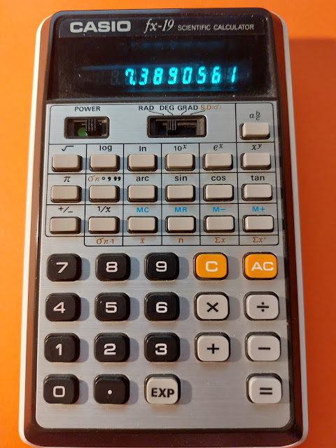
Retro Review: Casio fx-19

Retro Review: Casio fx-19

Quick Facts

Model: fx-19

Company: Casio

Production Years:  1976 - 1977

Power:  4 AA batteries.   AC adopter is available.

Type:  Scientific

Operating System:  Chain

Memory Registers:  1

Display:  One line:  8 digits or 5 digits with 2 digit exponent (10^xx)

Features and Keyboard

This is an early Casio scientific calculator with a standard set of features:

*  logarithm, antilogarithm (base 10 and e)

*  trigonometry

*  fractions (auto simplification)

*  one variable statistics

The fx-19 has 38 keys with two switches:  one for power and one for mode selection.  The mode selection switch has three angle modes (radians, degrees, grads) and one variable statistics (S.D σ).   

There is only one shift button, [ arc ], which is only for the inverse trigonometric functions arcsin, arccos, and arctan.  

Everything is displayed in floating point mode.  

Statistics Mode

In statistics mode, a lot of the keys are repurposed:

[ AC ]:   clear all statistical data

[ = ]:  enter statistical data 

[ ° ' '' ] ( σn ):  population deviation

[ 1/x ] ( σn-1 ): standard deviation

[ MC ] ( x-bar ):  mean 

[ MR ] ( n ):  number of data points

[ M- ] ( Σx ): sum of data points

[ M+ ] (Σx^2 ): sum of the square of data points

Example:  

Data Set:  { .786, .869, .542, .599, .649 }

In SD mode, 

[ AC ] .786 [ = ] .869 [ = ] .542 [ = ] .599 [ = ] .649 [ = ]

[ ° ' '' ] ( σn ):  0.120928

[ 1/x ] ( σn-1 ): 0.1352017

[ MC ] ( x-bar ):  0.689

[ MR ] ( n ):  5

[ M- ] ( Σx ): 3.445

[ M+ ] (Σx^2 ): 2.446723

Chain Mode

As we can tell from the pictures, there are no parenthesis keys.   The calculator operates in chain mode, which means the order of operations are not followed.   

In the following examples, the Degrees mode is set.  

Examples:

8 [ × ] 5 [ + ] 11 [ = ]  returns 51

5 [ + ] 8 [ × ] 11 [ = ]  returns 143

For complex calculations, often the use of the memory keys [ M+ ], [ M- ], [MR], and [ MC ] are needed.  Unfortunately, there is no indicator whether a non-zero number is in memory.   Hence, checking with the [ MR ] key is needed.   

Like many four-function regular calculations, [ M+ ] and [ M- ] complete pending operations.

Examples:

71 × 27 + 28 × 16 - 39 × 14

[ MC ]

71 [ × ] 27 [ M+ ]

28 [ × ] 16 [ M+ ]

39 [ × ] 14 [ M- ]

[ MR ]

Result:  1819

sin(30 + 0.05) / sin(30 - 0.05)

In division rational expressions, I prefer to tackle the denominator first.  

[ MC ] 

30 [ - ] .05 [ = ] [ sin ] [ M+ ]

30 [ + ] .05 [ = ] [ sin ] [ ÷ ] [ MR ] [ = ]

Result:  1.0030275

The Power Key

The power key [ x^y ] requires two arguments, the base (x) and the exponent (y).   When the power key is first press, the natural logarithm of x is displayed.

8^5

8 [ x^y ]    (Display:  2.0794415)

5 [ = ]     (Display:  32768)

The user of the power key is a treated as a separation calculation.   If we press any function for x, the power is canceled out.

6^(log 2)

Incorrect way:

6 [ x^y ] 2 [ log ] [ = ]

Result:   0.30103   (log 2)

Correct way:

[ MC ] 2 [ log ] [ M+ ]

6 [ x^y ] [ MR ] [ = ] 

Result:  1.7149319

The exception is roots, x [ x^y ] y [ 1/x ] [ = ]

7^(1/5)

7 [ x^y ] 5 [ 1/x ] [ = ]

Result:  1.4757732

Final Thoughts

The fx-19 is a classic calculator, and is a good option for those who want both a scientific calculator but operates more like a four-function calculator.   The fx-19 is still relatively available.   

Source

"Casio fx-19"  calculator.org.  

https://www.calculator.org/calculators/Casio_fx-19.html

Retrieved October 1, 2023

Eddie

All original content copyright, © 2011-2023.  Edward Shore.   Unauthorized use and/or unauthorized distribution for commercial purposes without express and written permission from the author is strictly prohibited.  This blog entry may be distributed for noncommercial purposes, provided that full credit is given to the author. 

 

Numworks: Polynomial Fit with Numpy (Software version 21 or later)

Numworks:  Polynomial Fit with Numpy  (Software version 21 or later)

The scripts polyfit.py and polyfitg.py perfectly fit a polynomial to a set of points.  For a set of n points, a polynomial of degree n-1 can be perfect fit to the set of points.   For instance,  2 points fit a perfect line,  3 points fit a quadratic polynomial, and 4 points fit a cubic polynomial.    Software version 21 or later is required as the numpy module is used.  

Numworks:  polyfit

polyfit.py:    Fit a number of points to a curve using the numpy module

403 bytes

from math import *

import numpy as np

# 2023-09-25 EWS

n=input("number of points? ")

n=int(n)

d=n-1

x=np.ones(n)

y=np.ones(n)

k=0

while k<n:

  print("point "+str(k+1))

  x[k]=float(input("x? "))

  y[k]=float(input("y? "))

  k+=1

p=np.polyfit(x,y,d)

# list coefficients

print("polynomial vector:")

print("x**n:  coef")

for k in range(n):

  print(str(n-k-1),":  ",str(p[k]))

print(p)

Numworks:  polyfitg

polyfitg.py:   Same as polyfit except a graph of the polynomial is drawn.   The coefficients are shown for 3 before the graph is drawn.  

743 bytes 

from math import *

from time import *

from matplotlib.pyplot import *

import numpy as np

# 2023-09-25 EWS

n=input("number of points? ")

n=int(n)

d=n-1

x=np.ones(n)

y=np.ones(n)

k=0

while k<n:

  print("point "+str(k+1))

  x[k]=float(input("x? "))

  y[k]=float(input("y? "))

  k+=1

p=np.polyfit(x,y,d)

# list coefficients

print("polynomial vector:")

print("x**n:  coef")

for k in range(n):

  print(str(n-k-1),":  ",str(p[k]))

print("\nplotting...")

sleep(3)

# graphing portion

c=(np.max(x)-np.min(x))/100

xc=[]

yc=[]

for i in range(101):

  xp=np.min(x)+i*c

  yp=np.polyval(p,xp)

  xc.append(xp)

  yc.append(yp)

axis((min(xc)-.5,max(xc)+.5,min(yc)-.5,max(yc)+.5)) 

axis(True)

grid(True)

plot(xc,yc,color="purple")

show()

Eddie

All original content copyright, © 2011-2023.  Edward Shore.   Unauthorized use and/or unauthorized distribution for commercial purposes without express and written permission from the author is strictly prohibited.  This blog entry may be distributed for noncommercial purposes, provided that full credit is given to the author. 

HP 15C: Transition Matrix Test and Taking a Square Matrix to an Integer Power

HP 15C:   Transition Matrix Test and Taking a Square Matrix to an Integer Power

Transition Matrix Test - Markov Chain

Let A be a square matrix of probabilities (entries from 0 to 1).   Is the square matrix suitable to be used in Markov Chain calculations?   It would qualify if for each row, the elements of that row have a sum to 1.  

The program:  

*  Tests whether Matrix A is a square matrix.  Non-square matrices are not transition matrices qualified for Markov Chains.   (lines 005 through 007)

*  Sum the elements of each row.

*  Tests whether sum of each row is 1. (LBL 2)

If (I) and (III) are met, then Matrix A is qualified to be used as a transition matrix for Markov Chain calculations.   This test returns a 1 for yes and 0 for no.

Store the contents and dimensions of Matrix A before running the program. 

HP 15C Program - Transition Matrix Test

Code:

001 : 42,21,11 : f LBL A

002 : 45,16,11 : RCL MATRIX A

003 : 36 : ENTER

004 : 36 : ENTER

005 : 45,23,11 : RCL DIM A

006 : 43,30, 6 :  g TEST 6  (x≠y)

007 : 22, 1 : GTO 1

008 : 44, 2 : STO 2

009 : 43,35 : g CLx

010 : 1 : 1

011 : 42,23,12 :  f DIM B

012 : 44,16,12 : STO MATRIX B

013 : 33 :  R↓

014 : 33 :  R↓

015 : 45,16,12 : RCL MATRIX B

016 : 42,26,13 : f RESULT C

017 : 20 : ×

018 : 42,16, 1 : f MATRIX 1

019 : 42,21, 2 : LBL 2

020 : 45, 2 : RCL 2

021 : 44, 0 : STO 0

022 : 45,13 : RCL C

023 : 1 : 1

024 : 43,30, 6 : g TEST 6 (x≠y)

025 : 22, 1 : GTO 1

026 : 42, 5, 2 : DSE 2

027 : 22, 2 : GTO 2

028 : 43,32 : RTN   (test passes)

029 : 42,21, 1 : f LBL 1  

030 : 43,35 : g CLx

031 : 43,32 : RTN  (test fails)

Notes:

RCL C instead of RCL MATRIX C is used because we want to recall the element, not the entire matrix.  The element that is recalled depends on the row (stored in R0) and column (stored in R1). 

HP 15C:  Square Matrix to a Positive Integer

Using a loop is required.  We are not able to use the x^2 or the y^x function with matrices, an Error 1 condition occurs.  

 A square matrix is stored in Matrix A.   Enter the positive integer power (n > 1) on the X stack before running the program.  

Code:  

032 : 42, 21, 11 : f LBL B

033:  1 :  1

034: 30 : -

035 : 44, 2 : STO 2

036 : 45,16,11 : RCL MATRIX A

037 : 44,16,12 : STO MATRIX B

038 : 42,21, 3 : f LBL 3

039 : 42,16,11 : f RESULT C

040 : 45,16,11 : RCL MATRIX A

041 : 45,16,12 : RCL MATRIX B

042 : 20 : ×

043 : 44,16,12 : STO MATRIX B

044 : 42, 5, 2 : f DSE 2

045: 22, 3 : GTO 3

046 : 45,16,13 : RCL MATRIX C

047: 42,16, 1 : f MATRIX 1

048 :43,32 : g RTN

Notes:  

MATRIX 1:  Set the row and column pointers to 1  (R0 = 1, R1 = 1)

Example

A = [ [ 0.3, 0.7, 0 ] [ 0.3, 0.3, 0.4 ] [ 0.2, 0.5, 0.3 ] ] 

GTO A R/S:   1  (yes, Matrix A is qualified for as a transition matrix)

If we insert a high enough power (as n → ∞), the matrix settles into a steady state, where each column will have the same value.

25 GTO B R/S:   C 3 x 3 

MATRIX 1

RCL C...

[ [ 0.2736, 0.4623, 0.2642 ] [ 0.2736, 0.4623, 0.2642 ] [ 0.2736, 0.4623, 0.2642 ] ]

Eddie

All original content copyright, © 2011-2023.  Edward Shore.   Unauthorized use and/or unauthorized distribution for commercial purposes without express and written permission from the author is strictly prohibited.  This blog entry may be distributed for noncommercial purposes, provided that full credit is given to the author. 

HP 15C: Vector Operations

HP 15C:   Vector Operations

Calculators covered:

* HP 15C

* HP 15C Limited Edition

* HP 15C Collector's Edition

* Apps, Swiss Micros DM 15

HP 15C:   Dot Product, Tensor Product, and Angle Between Vectors

Set vectors A and B as 3 x 1 vectors (3 rows, 1 column)

3 ENTER 1 dim A

3 ENTER 1 dim B

Dot Product  (LBL D)  

Dot product:  A ⋅ B = A^T B 

The result is a single number.

Code: 

001 : 42,21,14 : LBL D

002 : 45,16,11 : RCL MATRIX A

003 : 42,16, 4 : MATRIX 4

004 : 45, 16, 12 : RCL MATRIX B

005 : 42, 26, 13 : RESULT C

006 : 20 : ×

007 : 45,16,11 : RCL MATRIX A

008 : 42,16, 4 : MATRIX 4

009 : 45,13 : RCL C

010 : 43,32 : RTN

Tensor Product (LBL E)

Tensor product:  A ⊗ B = A B^T

The result is a 3 x 3 matrix

Code: 

011 : 42,21,15 : LBL E

012 : 45,16,11 : RCL MATRIX A

013 : 45,16,12 : RCL MATRIX B

014 : 42,16, 4 : MATRIX 4

015 : 42,26,13 : RESULT C

016 : 20 : ×

017 : 45,16,12 : RCL MATRIX B

018 : 41,16, 4 : MATRIX 4

019 : 42,16, 1 : MATRIX 1

020 : 45,16,13 : RCL MATRIX C

021 : 43, 32 : RTN

Angle Between Vectors (LBL 0)

θ = arccos( (A ⋅ B) ÷ (||A|| ||B||) )

Code:

022 : 42,21, 0 : LBL 0

023 : 32,14 : GSB D

024 : 45,16,11 : RCL MATRIX A

025 : 42,16, 8 : MATRIX 8

026 : 45,16,12 : RCL MATRIX B

027 : 42,16, 8 : MATRIX 8

028 : 20 : ×

029 : 10 : ÷

030 : 43,24 : COS^-1

031 : 43,32 : RTN

Notes:  

MATRIX 4:  Transposes a matrix, which it is stored in the original matrix slot.  

MATRIX 8:  The 2-norm of a matrix.   It is calculated by taking a square root of the sum of the square of each element.  √(Σ( A_r,c ^ 2,  r = 1 to n and c = 1 to m))

For the dot and tensor products, I transpose the appropriate matrix back to the 3 x 1 form after the calculation.

Example

A = [ [ 4 ], [ 5 ], [ -2 ] ]

B = [ [ -3 ], [ 9 ], [ 8 ] ]

Dot Product:  GTO D R/S

Result:  17

Tensor Product:   GTO E R/S

Result:

[ [ -12, 36, 32 ], [ -15, 45, 40 ], [ 6, -18, -16 ] ]

Angle Between Vectors:  GTO 0 R/S

Result:  78.2166°

Eddie

All original content copyright, © 2011-2023.  Edward Shore.   Unauthorized use and/or unauthorized distribution for commercial purposes without express and written permission from the author is strictly prohibited.  This blog entry may be distributed for noncommercial purposes, provided that full credit is given to the author. 

HHC 2023 Conference Videos

 HHC 2023 Conference Videos

The annual HP Handheld Conference took place on October 7 and 8, 2023 in Orlando.  Unfortunately, I couldn't make it because I was recovering from surgery.

The conference had a record high number of presentations by calculator enthusiasts, Hewlett Packers, distributors and partners Royal and Moravia.  

The list presented is what is available on the hpcalc.org's YouTube page as of today - but there is definitely more to come:

What's New in the HHC 2023 USB Drive - Eric Rechlin

You can order a drive for $65 from hpcalc.org's commerce page:  

https://commerce.hpcalc.org/hhcusb.php

Shipping to begin at late October.  Disclaimer:  I am not receiving any compensation for this; this is to promote the HHC conference.

HP Inc Partner Update (Mitch Abrams)

Royal Partner Update (David Joachim)

Moravia Partner Update (Klaas Kuperus and Radim Frydrych)

Recreating the HP 15c Handbooks (Eric Rechlin)

25 Years of the PPC Archive (Jack Schwartz)

HP Portable Plus DRam ROM Development Module (Chuck McCord)

Things the HP-41 Designers Got Wrong (Gene Wright)

CC41 Decimated (Craig Bladow)

Conference web page:

https://hhuc.us/2023/index.htm

Gratitude to hpcalc.org and I plan to make it HHC 2024!  

Eddie

All original content copyright, © 2011-2023.  Edward Shore.   Unauthorized use and/or unauthorized distribution for commercial purposes without express and written permission from the author is strictly prohibited.  This blog entry may be distributed for noncommercial purposes, provided that full credit is given to the author. 

HP 32SII: Glide Slope Calculations (and Memory Management)

HP 32SII:  Glide Slope Calculations (and Memory Management)

Note:   These programs should work on the Swiss Micros DM32.  

Introduction

The following program calculates the forces and angle for a flight of a glider, an aircraft without a engine:

*  Weight

*  Lift Force

*  Drag Force

SI units are used.

With inputs glide distance (G), height (H), and mass (M):

Angle:  A = arcsin(H ÷ G)

Weight:  W = M × 9.80665

Lift:  L = W × sin A

Drag:  D = W × cos A

The program uses the polar-to-rectangular conversion to calculate lift and drag. 

HP 32SII Programs:  Glide Slope Calculations

Code 1:

G01  LBL G

G02  DEG

G03  INPUT G

G04  INPUT H

G05  INPUT M

G06  R↓

G07  x<>y

G08  ÷

G09  ASIN

G10  STO A

G11  VIEW A

G12  R↑

G13  9.80665

G14  ×

G15  STO W

G16  VIEW W

G17  θ,r→y,x

G18  STO L

G19  VIEW L

G20  x<>y

G21  STO D

G22  VIEW D

G23  RTN

Bytes:  42.5

Checksum:  4717

Notes:

*  This version has prompts and view commands to guide the user.  We don't have to preload registers as the INPUT commands guide us.

*  All inputs and outputs are stored to variables.   7 variables are used, which will require 56 bytes.  On the HP 32SII, each variable that contains non-zero values takes 8 bytes of memory.  If you want to make the variables local, insert a CLVARS command for G23 and line G24 becomes RTN.

Variables:

Input:

G = Glide Distance.  The distance that glider climbs to it's peak.   Think of the hypotenuse of a right triangle.   Distance is in meters.  

H = Height.  The height that the glider reaches.  Distance is in meters.

M = Mass.  Mass of the glider in kilograms.

Output:

A = Angle.  Angle of the of glider's flight in degrees. 

W = Weight.  Weight of the glider, which is Newtons.

L = Lift force of the glider, in Newtons.

D = Drag force of the glider, in Newtons.

Code 2:

Code 2 is a shorter code which does not store anything into variables.   The program starts with G (glide distance), H (height), and M (mass) on the stack.  

L01   LBL L

L02   DEG

L03   R↓

L04   x<>y

L05   ÷

L06   ASIN

L07   STOP  (display A)

L08   R↑

L09   9.80665

L10   ×

L11   STOP  (display W)

L12   θ,r→y,x

L13   RTN    (L is on the x stack, D is on the y stack)

Bytes:  27.5 bytes

Checksum:  6446

Examples

Example 1:

Glider distance:  G = 178 m

Height:  H = 23 m

Mass of the glider:  M = 55 kg

Output:

Angle:  A ≈ 7.4241°

Weight:  W ≈ 539.3658 N

Lift:  L ≈ 534.8441 N

Drag:  D ≈ 69.6933 N

Example 2: 

Glider distance:  G = 200 m

Height:  H = 30 m

Mass of the glider:  M = 39 kg

Output:

Angle:  A ≈ 8.6269°

Weight:  W ≈ 382.4594 N

Lift:  L ≈ 378.1322 N

Drag:  D ≈ 57.3689 N

Source

National Museum of the United States Air Force.  "Mathematics of Flight:  Glide Slope II"  September 2020.  Retrieved August 2023.   

https://www.nationalmuseum.af.mil/Portals/7/Mathematics%20of%20Flight%20Glide%20Slope%20II.pdf

Eddie 

All original content copyright, © 2011-2023.  Edward Shore.   Unauthorized use and/or unauthorized distribution for commercial purposes without express and written permission from the author is strictly prohibited.  This blog entry may be distributed for noncommercial purposes, provided that full credit is given to the author. 

TI-84 Plus CE Python and Numworks Python: Color Contrast

 TI-84 Plus CE Python and Numworks Python:  Color Contrast

Introduction and Calculation

The following Python script compares a contrast of colored text (foreground) color against a background color.  It is important to have good, high contrast.  High contrast allows for easy readability and it's easier on the eyes.   This becomes more important when considering web page development to allow accessibility.  

Steps:

1.  Get the RGB color code for the background color.  Here the decimal values of 0-255 are used.   R is red, G is green, and B is blue.   Black has all three entered as 0.  White has all three values entered as 255.  

2.  Take the ratio of each color out of 255 as such:

x = x ÷ 255

Where x stands for R, G, and B.  Do this for each color.  We want to the decimal answer, not the percentage.  

3.  For each color (R, G, B), do this calculation:

If x ≤ 0.03928

Then x = x ÷ 12.92

Else x = ((x + 0.055) ÷ 1.055)^2.4

Again, x stands for R, G, and B.  Do this for each color.

4.  Calculate the luminosity as:

L = 0.02126 * R + 0.7152 * G + 0.0722 * B

Let l1 = L (background color).

5.  Do steps 1-4 for the text color.  Let l2 = L (text color).

6.  Set the light color as the maximum between the background color and text color.  Set the dark color as the minimum between the background color and text color.  The contrast is calculated as follows:

c = (light + 0.05) ÷ (dark + 0.05)

If c = 21, you have perfect contrast.  If c = 1, you have the worst contrast.  Hence, we want as high contrast as possible.  This is one measure of how good colors compare to each other.  

The script presented is for the TI-84 Plus CE Python (and TI-83 CE Premium Python Edition) and Numworks. There are slight differences between the scripts, which will be highlighted in each section.

TI-84 Plus CE Python script:  CNTRST84.py

Notes:

The Texas Instruments version uses the following modules:  math, ti_system, and ti_draw.   

The ti_system has the wait_key() command, which allows us to stop the program execution until a key is pressed.

Code:

from math import *

from ti_system import *

from ti_draw import *

# 2023-08-12 EWS

# Contrast - TI-84 Plus CE Python Version

# Source:

# www.w3.org, "WCAG 2.0"

# ADG*, "How to calculate colour contrast"

# CODE:

# subs

def lumin(r,g,b):

  r=compare(r/255)

  g=compare(g/255)

  b=compare(b/255)

  return .2126*r+.7152*g+.0722*b

def compare(x):

  if x<=.03928:

    x=x/12.92

  else:

    x=((x+.055)/1.055)**2.4

  return x

# main

print("Color Contrast \n(0-255) \nBackground color:")

r1=int(input("red? "))

g1=int(input("green? "))

b1=int(input("blue? "))

print("Text color:")

r2=int(input("red? "))

g2=int(input("green? "))

b2=int(input("blue? "))

# calc

l1=lumin(r1,g1,b1)

l2=lumin(r2,g2,b2)

cntr=(max(l1,l2)+.05)/(min(l1,l2)+.05)

print("Contrast: ",str(cntr))

# pause the screen

k=0

while k==0:

  k=wait_key()

# draw

clear()

set_color(r1,g1,b1)

fill_rect(0,0,319,200)

set_color(r2,g2,b2)

draw_text(25,65,"Contrast test: TI-84+ CE")

draw_text(25,125,"Press clear to continue.")

show_draw()

Numworks script:  CNTRSTNW.py

Notes:

The Nuwmorks version uses the following modules:   math and kandinsky.  The kandinsky module is one of the graphics modules Numworks has.  

Due to a lack of a get key command, I have decided to display both the contrast and the color test as the last step.  The calculated contrast will always be printed with black text on white background.

Code:

from math import *

from kandinsky import *

# 2023-08-13 EWS

# Contrast - Numworks Version

# Source:

# www.w3.org, "WCAG 2.0"

# ADG*, "How to calculate colour contrast"

# CODE:

# subs

def lumin(r,g,b):

  r=compare(r/255)

  g=compare(g/255)

  b=compare(b/255)

  return .2126*r+.7152*g+.0722*b

def compare(x):

  if x<=.03928:

    x=x/12.92

  else:

    x=((x+.055)/1.055)**2.4

  return x

# main

print("Color Contrast \n(0-255) \nBackground color:")

r1=int(input("red? "))

g1=int(input("green? "))

b1=int(input("blue? "))

print("Text color:")

r2=int(input("red? "))

g2=int(input("green? "))

b2=int(input("blue? "))

# calc

l1=lumin(r1,g1,b1)

l2=lumin(r2,g2,b2)

cntr=(max(l1,l2)+.05)/(min(l1,l2)+.05)

# draw

c1=color(r1,g1,b1)

c2=color(r2,g2,b2)

cb=color(0,0,0)

cw=color(255,255,255)

fill_rect(0,0,320,240,c1)

draw_string("Contrast test: Numworks",25,25,c2,c1)

draw_string("Contrast: "+str(cntr),25,50,cb,cw)

draw_string("Press OK to continue.",25,150,c2,c1)

Sources

"How to calculate colour contrast"  Accessibility Developer Guide (ADG*).  An initiative of Access for all.  Last Edited July 29, 2023.  Accessed August 8, 2023.

https://www.accessibility-developer-guide.com/knowledge/colours-and-contrast/how-to-calculate/

"Relative Luminance" Web Content Accessibility Guidelines (WCAG) 2.0.   W3C, Inc.  (World Wide Web Consortium, Inc.)   Last Edited December 11, 2008.  Accessed August 8, 2023.   https://www.w3.org/TR/WCAG20/#relativeluminancedef

Eddie 

All original content copyright, © 2011-2023.  Edward Shore.   Unauthorized use and/or unauthorized distribution for commercial purposes without express and written permission from the author is strictly prohibited.  This blog entry may be distributed for noncommercial purposes, provided that full credit is given to the author. 

TI-84 Plus CE: Using Matrices for "Tax Table" Calculations

TI-84 Plus CE:   Using Matrices for "Tax Table" Calculations

How The Matrix is Set Up

Each row represents a tier or a bracket.  

First column:  Lower Limit.  This is the test variable.  The first tier often will have the lower tier of 0.

Second and subsequent columns:    Variables that are associated with that tier.

Let's demonstrate this with an example.

Example Tax Bracket

This matrix has four brackets (four rows).  The algorithm starts with the last (bottom) row and tests whether the input is greater or equal to the test variable.  

According to the table, the tax rate changes at income level at $30,000, $90,000, and $270,000, with the top tax rate of 9% effective for all income excess of $270,000.

If the income is $29,999.99, the first tier of 3% is used.  If the income goes to $30,000.00, the next tier is activated.

The program ITAX, which uses this type of setup, goes "backwards".  It tests from the highest tier down.  

For example:  Income = $50,000

Start at tier 4 (bottom row). 

Is 50,000 > 270,000?  No, go to tier 3. (move one row up)

Is 50,000 > 90,000?  No, go to tier 2.  (move one row up) 

Is 50,000 > 30,000?  Yes, use the variables from tier 2.

Tax:  (50,000 - 30,000) × 5% + 900 = 20,000 × 5% + 900 = 1,900

Matrix wise:   (income - M[2,1]) * M[2,2] ÷ 100 + M[2,3]

Programs

There are two programs that illustrate this method:  

ITAX:  Income Tax Bracket.  Bracket is stored in Matrix [ A ] and has three columns:

Column 1:  lower limit of each bracket

Column 2:  tax rate for that bracket

Column 3:  additional "minimum" tax.   

BAROMET:  Calculates the air pressure and density based on height.  Scientific information is stored in Matrix [ J ].  

Column 1:  height in meters

Column 2:  mass density in kg/m^3

Column 3:  standard temperature in K

Column 4:  static pressure in Pa

If you are working in US Units, the height is converted to meters first.  After the calculation, the results are converted back into US units. 

You can download both programs here (zip file):  

https://drive.google.com/file/d/1ZCtMcJgZDLUGnrAHE6cPAkWBQQj1aHKc/view?usp=sharing

Source

"Barometric formula."  Wikipedia.  Last edited July 13, 2023.  Retrieved July 16, 2023.   https://en.wikipedia.org/wiki/Barometric_formula

Eddie

All original content copyright, © 2011-2023.  Edward Shore.   Unauthorized use and/or unauthorized distribution for commercial purposes without express and written permission from the author is strictly prohibited.  This blog entry may be distributed for noncommercial purposes, provided that full credit is given to the author. 

TI 84 Plus CE Python and Numworks - Cosine Similarity

 TI 84 Plus CE Python and Numworks  - Cosine Similarity

Note:  The python script should work on the TI-83 Premium CE Python Edition, TI-Nspire CX II, Casio fx-9750GIII, and Casio fx-CG 50. The script only calls for the math module, which is standard on all platforms.  

Introduction and Calculating the Cosine Similarity

We can find how similar two phrases by calculating the cosine similarity.  This is similar to finding the angle between two vectors.  

Here are the steps:

1.  Separate the phrases into a list of words.   In Python, this can easily achieved by .split() attachment.  We can split using any character, but if the argument is left blank, the character used is the space.

Example:

str1="here comes the sun"

list1=str1.split()

print(list1) 

Output:

['here', 'comes', 'the', 'sun']

2.  Return the unique elements of each list. That is, filter out any repeats. Since the program is using two lists, we need to combine the two list of words from the phrases and then filter out any repeated words.

Example:

list1=['my', 'apple', 'is', 'in', 'my', 'apple', 'pie']

u=[ ]

for i in list1:

  if i not in u:

    u.append(i)

print(u)

Output:

['my', 'apple', 'is', 'in', 'pie']

3.  Obtain a word count of each of two phrases compared to the unique list of words from two phrases combined.     The .count(arg) attachment to a list returns the number of occurrences of arg is present in that list.

Example:

list1=['my', 'apple', 'is', 'in', 'my', 'apple', 'pie']

list1.count('apple')

Output: 

2   

This step is accomplished by the list comprehension:

[lsrc.count(i) for i in lmain]

lsrc = source list

lmain = main list

We are counting the number of occurrences of each word in lmain found in lsrc.

The result are two equal-sized vectors of integers.

4.  Calculate the cosine similarity by the formula:

cos θ = dot(v1, v2) ÷ (norm(v1) × norm(v2))

dot(v1, v2):  the dot product of the count vectors

norm(v1) and norm(v2):  norm of the count vectors

The cosine similarity varies between 0 and 1.   We are not going to calculate θ itself.  Hence the cosine similarity (CS) is:

CS = dot(v1, v2) ÷ (norm(v1) × norm(v2))

For more details, please refer to the excellent "Cosine Similarity, Clearly Explained!!!" video from StatQuest, which is listed in the Sources below.  

Python Code:  cossim2.py

# phrases prograrm

# 2023-08-06 ews

from math import *

# subroutines

def unique(l):

  u=[]

  for i in l:

    if i not in u:

      u.append(i)

  return u

def counta(lmain,lsrc):

  c=[lsrc.count(i) for i in lmain]

  return c

def norm(v):

  # list have integers

  s=[i**2 for i in v]

  s=sqrt(sum(s))

  return s

# main program

print("\nDo not use punctuation")

str1=input("phrase 1? ")

str2=input("phrase 2? ")

# split into 2 lists

list1=str1.split()

list2=str2.split()

# find the unique list

list3=list1+list2

list3=unique(list3)

# word count

listc1=counta(list3,list1)

listc2=counta(list3,list2)

# vector operations

# norm

n1=norm(listc1)

n2=norm(listc2)

# dot

d=sum([listc1[i]*listc2[i] for i in range(len(listc1))])

# cosine similarity

c=d/(n1*n2)

# no need to take the arccosine

print("cosine similarity: ")

print(c)

print("\n0: no words in common \n1: all words in common")

Numworks page:    https://my.numworks.com/python/ews31415/cossim2

Download:  https://drive.google.com/file/d/1qOtHIau6vm_TolNQugjhHthnO3ECoe9d/view?usp=sharing

Examples

Phrase 1:   hello world

Phrase 2:  hi planet earth

Cosine Similarity:  0.0   (no words in common)

Phase 1:  girls like flowers and trees

Phase 2:  boys like trees and raccoons

Cosine Similarity:  0.5999999999998   (exact:  0.6)

When entering phrases, do not use punctuation.   I would just use all lowercase or all uppercase for the most accurate results.   The matches are exact, so spelling counts!  

Sources

Infopedic Techie.  "Python program to find the unique values in a list || Python list [example-3]".   YouTube video posted on March 7, 2019.  https://www.youtube.com/watch?v=7f2UJgig2yI

StatQuest with Josh Starmer.  "Cosine Similarity, Clearly Explained!!!"  YouTube video posted on January 29, 2023.

https://www.youtube.com/watch?v=e9U0QAFbfLI

"Cosine Similarity"  Wikipedia.  Last edited July 6, 2023, accessed August 2023.

https://en.wikipedia.org/wiki/Cosine_similarity

Eddie

All original content copyright, © 2011-2023.  Edward Shore.   Unauthorized use and/or unauthorized distribution for commercial purposes without express and written permission from the author is strictly prohibited.  This blog entry may be distributed for noncommercial purposes, provided that full credit is given to the author.