Casio fx-CG 50: Draw a Polygon of Vertices

Casio fx-CG 50: Draw a Polygon of Vertices 

Introduction

The program POLYPTS draws a polygon of vertices and calculates the area.

Casio fx-CG 50 Program: POLYPTS

ClrGraph

S-WindAuto

“# POINTS”? → N

(1 + N) → Dim List 1

(1 + N) → Dim List 2

For 1 → I to N

ClrText

Green Locate 1, 7, “POINT”

Red Locate 7, 7, I

“X”? → List 1[ I ]

“Y”? → List 2[ I ]

Next

List 1[ 1 ] → List 1[N + 1]

List 2[ 1 ] → List 2[N + 1]

0 → A

For 2 → I To N+1

A + (List 1[ I ] × List 2[I – 1] – List 1[I – 1] × List 2[ I ]) → A

Next

Abs A ÷ 2 → A

“AREA = “

A ◢

S-Gph 1 DrawOn, xyLine, List 1, List 2, 1, Square, ColorLinkOff, ColorAuto

DrawStat

Examples

Example 1: 4 Points

(0, 14)

(5, 5)

(18, 0)

(0, -4)

Area = 116

Example 2: 4 Points

(4, 10)

(15, 10)

(11, 2)

(2, 2)

Area = 80

Example 3: 5 Points

(1, 1)

(4, 2)

(3, 6)

(0, 4)

(0, 2)

Area = 13

Next time, an anniversary for the blog...  14 years!   Gratitude as always,

Eddie

All original content copyright, © 2011-2025. Edward Shore. Unauthorized use and/or unauthorized distribution for commercial purposes without express and written permission from the author is strictly prohibited. This blog entry may be distributed for noncommercial purposes, provided that full credit is given to the author.

HP Prime: Minimum Distance Between a Point and a Line

HP Prime: Minimum Distance Between a Point and a Line

Introduction

We have a line in the form of y = m * x + b, where m is the slope of the line and b is the y-intercept of the line, and a separate point (px, py). The task is to find the minimum distance, or the shortest distance, between the point and the line. The separate point is not required to be on the line. The line and point are in two-dimensional space.

If the point (px, py) is not on the line, then theoretically, there are an infinite amount of distances between the point and the line. However, to get the shortest distance, draw a path that is “directly straight” to the line. This is achieved by choosing a line that connects the (px, py) that is a line that is orthogonal (perpendicular) to the line y = m * x + b.

The line drawn is of the form y = -1/m * x + b1. The slope of the orthogonal line is -1/m. Assuming that m ≠ 0, the y-intercept of the orthogonal line is b1 = y1 + x1 / m.

The next step is to find where the two lines intersect, which is done by solving the following system for x and y:

y = m * x + b

y = -m / n + b1

Label the intersection point (x1, y1). The minimum distance will be calculated as follows:

dist = √( (x1 – px)^2 + (y1 – py)^2 ) = abs( (x1 – px) + (y1 – py)*i)

If m = 0, the line is in the form of y = b. The orthogonal line is x = px, and the distance is simply abs( (y1 – py)*i ).

HP Prime Code: PTLNDIST

EXPORT PTLNDIST()

BEGIN

// 2024-07-21 EWS

// radian

HAngle:=0;

LOCAL px,py,m,b;

INPUT({m,b,px,py},

"Point-Line Distance (px, py), y=mx+b",

{"m:","b:","px:","py:"},

{"m: slope"," b: y-intercept",

"point x","point y"});

LOCAL y0;

y0:=m*px+b;

LOCAL b1,mt,x1,y1,dist,str;

IF m≠0 THEN

b1:=py+px/m;

mt:=[[−m,1],[1/m,1]]^-1*[[b],[b1]];

x1:=mt[1,1];

y1:=mt[2,1];

dist:=ABS((x1-px)+(y1-py)*√(-1));

ELSE

x1:=px;

y1:=b;

dist:=ABS((y1-py)*√(-1));

END;

// print results

PRINT();

PRINT("Results:");

PRINT("Intersect point:");

PRINT("x: "+STRING(x1));

PRINT("y: "+STRING(y1));

PRINT("");

IF m≠0 THEN

str:="Y="+STRING(-1/m)+"*X+"+STRING(b1);

ELSE

str:="X="+STRING(x1);

END;

PRINT("Orthogonal Line:");

PRINT(str);

PRINT("");

PRINT("Minimum Distance:");

PRINT(dist);

RETURN {x1,y1,str,dist};

END;

Note:

√(-1) represents the imaginary number ⅈ ( [ Shift ], [ 2 ] ).

Inputs:

* The slope of the y-intercept of the line y = m * x + b (no vertical lines, but m can be zero)

* The point (px, py)

Outputs:

* The line that runs through point (px, yx) that is orthogonal to y = m * x + b. The slope and y-intercept of the orthogonal line, which the line will be stated in a string

* The intersection point of the two lines.

* The distance between (px, yx) and the intersection point. (dist)

Examples

Example 1:

Inputs: Line: y = 5 x – 2, Point: (-1, -5)

m = 5

b = -2

px = -1

py = -5

Results:

Intersect point:

x = -0.615384615386

y = -5.07692307692

Orthogonal Line:

Y = -0.2 * X – 5.2

Minimum distance:

0.392232270274

Example 2:

Inputs: Line: y = 6, Point: (3, -9)

m = 0

b = 6

px = 3

py = -9

Results:

Intersect point:

x = 0.764705882353

y = 4.05882352941

Orthogonal Line:

X = 3

Minimum distance:

15

Example 3:

Inputs: Line: y = 4 x + 1, Point: (5, 3)

m = 4

b = 1

px = 5

py = 3

Results:

Intersect point:

x = 0.764705882353

y = 4.05882352941

Orthogonal Line:

Y = -0.25 * X + 4.25

Minimum distance:

4.36564125066

Source

Tremblay, Christopher. Mathematics for Game Developers. Thomson Course Technology. Boston, MA. 2004. ISBN 1-59200-038-X.

Eddie

All original content copyright, © 2011-2024. Edward Shore. Unauthorized use and/or unauthorized distribution for commercial purposes without express and written permission from the author is strictly prohibited. This blog entry may be distributed for noncommercial purposes, provided that full credit is given to the author.

Casio fx-CG 50: Points on a Circle

 Casio fx-CG 50: Points on a Circle

Introduction and Derivation

Given the initial point on a circle (x, y). If the point travels on a circle a distance of arc length s, where is the new point on the circle? Assumption: The center of the circle lies on the point (0, 0).

In fact, we can have two points depending on the direction traveled: counter-clockwise or clockwise. The programs presented today will determine both points.

Points that lie on the circle have the same radius. Determine the required radius:

r = √(x^2 + y^2)

And since the circle is centered at (0, 0), we can determine the angle by:

θ = arctan(y/x) = arg(x + yi)

We will assume all angles are in radians.

The arc length can be used to determine the angle traveled. Let’s call this angle z:

s = r × z

z = s / r

The new points can be determined by:

x’ = r × cos(θ + z), y’ = r × sin(θ + z)

x’’ = r × cos(θ - z), y’’ = r × sin(θ - z)

Casio fx-CG 50 Basic: PTSONCIRC

Code:

ClrText

Blue “POINTS ON”

Blue “THE CIRCLE”

Blue “CENTER (0,0)”

Red “RADIANS”

Rad

“INITIAL X”? → X

“INITIAL Y”? → Y

“ARC LENGTH”? → S

Abs (X+Yi) → R

Arg (X+Yi) → θ

S ÷ R → Z

R × cos(θ + Z) → A

R × sin(θ + Z) → B

R × cos(θ - Z) → C

R × cos(θ - Z) → D

ClrText

Green Locate 1,3,”POINT 1”

Black Locate 1,4,A

Blue Locate 11,4,”,”

Black Locate 12,4,B

Green Locate 1,5,”POINT 2”

Black Locate 1,6,C

Blue Locate 11,6,”,”

Black Locate 12,6,D

For monochrome models, leave out the color commands (Blue, Red, Black, Green)

Casio fx-CG 50 Python: ptsoncirc.py

Code:

from math import *

print(“Points on\nthe circle.”)

print(“Center is at (0,0)”)

x=float(input(“initial x? “))

y=float(input(“initial y? “))

s=float(input(“arc length? “))

r=sqrt(x**2+y**2)

t=atan(x,y)

z=s/r

b,a=r*cos(t+z),r*sin(t+z)

d,c=r*cos(t-z),r*sin(t-z)

print(“Point 1”)

print(str(a),”,\n”,str(b))

print(“Point 2”)

print(str(c),”,\n”,str(d))

Examples

X: 5, Y: 6, S: 1.5

Point 1: (3.76280901, 6.84406811)

Point 2: (6.05333094, 4.93529983)

X: 4: Y: 5, S: 1

Point 1: (3.173620164, 5.561306956)

Point 2: (4.729016994, 4.316989492)

Python Pointers

Storing to Multiple Variables in One Line

We can store a value to multiple variables in one line. For example,

a = b = 7

Stores the value 7 to both the variables a and b.

We can store multiple values to multiple values to multiple variables in one line. For example:

a, b = 7, 8

Stores 8 to the variable b and 7 to the variable a. The expression works from the inside-out.

We could also have both uppercase and lowercase letters as different variables, such as A and a. I choose not to because I want to avoid confusion.

New Line Escape Character: \n

In a string, we can add \n (backslash, n) to create a new line.

Eddie

All original content copyright, © 2011-2024. Edward Shore. Unauthorized use and/or unauthorized distribution for commercial purposes without express and written permission from the author is strictly prohibited. This blog entry may be distributed for noncommercial purposes, provided that full credit is given to the author.

Numworks: Polynomial Fit with Numpy (Software version 21 or later)

Numworks:  Polynomial Fit with Numpy  (Software version 21 or later)

The scripts polyfit.py and polyfitg.py perfectly fit a polynomial to a set of points.  For a set of n points, a polynomial of degree n-1 can be perfect fit to the set of points.   For instance,  2 points fit a perfect line,  3 points fit a quadratic polynomial, and 4 points fit a cubic polynomial.    Software version 21 or later is required as the numpy module is used.  

Numworks:  polyfit

polyfit.py:    Fit a number of points to a curve using the numpy module

403 bytes

from math import *

import numpy as np

# 2023-09-25 EWS

n=input("number of points? ")

n=int(n)

d=n-1

x=np.ones(n)

y=np.ones(n)

k=0

while k<n:

  print("point "+str(k+1))

  x[k]=float(input("x? "))

  y[k]=float(input("y? "))

  k+=1

p=np.polyfit(x,y,d)

# list coefficients

print("polynomial vector:")

print("x**n:  coef")

for k in range(n):

  print(str(n-k-1),":  ",str(p[k]))

print(p)

Numworks:  polyfitg

polyfitg.py:   Same as polyfit except a graph of the polynomial is drawn.   The coefficients are shown for 3 before the graph is drawn.  

743 bytes 

from math import *

from time import *

from matplotlib.pyplot import *

import numpy as np

# 2023-09-25 EWS

n=input("number of points? ")

n=int(n)

d=n-1

x=np.ones(n)

y=np.ones(n)

k=0

while k<n:

  print("point "+str(k+1))

  x[k]=float(input("x? "))

  y[k]=float(input("y? "))

  k+=1

p=np.polyfit(x,y,d)

# list coefficients

print("polynomial vector:")

print("x**n:  coef")

for k in range(n):

  print(str(n-k-1),":  ",str(p[k]))

print("\nplotting...")

sleep(3)

# graphing portion

c=(np.max(x)-np.min(x))/100

xc=[]

yc=[]

for i in range(101):

  xp=np.min(x)+i*c

  yp=np.polyval(p,xp)

  xc.append(xp)

  yc.append(yp)

axis((min(xc)-.5,max(xc)+.5,min(yc)-.5,max(yc)+.5)) 

axis(True)

grid(True)

plot(xc,yc,color="purple")

show()

Eddie

All original content copyright, © 2011-2023.  Edward Shore.   Unauthorized use and/or unauthorized distribution for commercial purposes without express and written permission from the author is strictly prohibited.  This blog entry may be distributed for noncommercial purposes, provided that full credit is given to the author. 

TI-84 Plus CE Python: Polygon Path (ppath.py)

TI-84 Plus CE Python:  Polygon Path (ppath.py)

Introduction

The program PPATH:

Between two points:  

1.  Calculates the required leftward, counter-clockwise angle.

2.  Calculates the distance to be traveled. 

The path starts at the origin (0,0).  You can create open paths or closed polygons.  For polygons, add another point and include (0,0) as the last point.  

TI-84 Plus CE Python Program:  PPATH - Python (ppath)

Download the TI-84 Plus CE Python file here:  https://drive.google.com/file/d/1QnPP9ikx45i7gAH22fTkFAmE-pBFQwTD/view?usp=sharing

Copy the code for a text file.  

print("Poly Path \nEdward Shore")

# 2022-04-27

from math import *

from turtle import *

t=Turtle()

# t is required for turtle

from ti_system import *

# hide the grid

t.hidegrid()

# obtain the points

x=[0]

y=[0]

# angles

g=[0]

# degree difference

q=[0]

# distance

d=[0]

print("Point 0: (0,0)")

print("#_0 to #_n-1")

n=eval(input("# points? "))

for i in range(1,n):  

  a=eval(input("x"+str(i)+"? "))

  b=eval(input("y"+str(i)+"? "))

  x.append(a)

  y.append(b)

  r=sqrt((a-x[i-1])**2+(b-y[i-1])**2)

  d.append(r)

  m=degrees(atan2(b-y[i-1],a-x[i-1]))

  v=m-g[i-1]

  if v<0:

    v+=360

  g.append(m)

  q.append(v)

  r6=round(r,6)

  m6=round(v,6)

  print("Distance: "+str(r6))

  print("Left Turn: "+str(m6)+"\u00b0")

print("\nPress [clear] to continue.")

disp_wait()

t.home()

t.pencolor(0,128,0)

# set speed

t.speed(4)

for i in range:

  t.left(q[i])

  t.forward(d[i])

t.done()

Notes:

1.  Turtle is a add-in module for the TI-84 Plus CE Python, which must be downloaded. Download the Turtle module here:  https://education.ti.com/en/product-resources/turtle-module/ti84ce-python

2.  Calling the Turtle module automatically assigns the variable t to a drawing turtle by the line t=Turtle().

3.  The ti_system module is exclusive to the TI-84 Plus CE.  This allows the program to pause with the disp_wait command.  

4.  The underscore character ( _ ) can be typed by the [ 2nd ] [ (-) ] (ans) sequence.  

5.  The hashtag character ( # ) can be typed by the [ 2nd ] [ 3 ] (L3) sequence.  

6.  The line for i in range(1,n) starts a for loop with i taking the values from 1 to n-1. This is good for lists when the initial point (point 0) does not need further processing. 

7.  The default operating angle measurement in Python is Radians.  

8.  The angle difference, which tells us how many degrees to turn left, is normalized to the 0°-360° range.   This is optional.   

9.  The line t.home() sets the turtle to point (0,0) and sets the turtle's orientation to 0° (facing right, forward on the x-axis).

10.  The line t.done() shows the results of the turtle commands. 

Examples

Example 1: Quadrilateral

Example 2:  An Open Path

Enjoy!  

Eddie 

All original content copyright, © 2011-2022.  Edward Shore.   Unauthorized use and/or unauthorized distribution for commercial purposes without express and written permission from the author is strictly prohibited.  This blog entry may be distributed for noncommercial purposes, provided that full credit is given to the author. 

HP Prime and TI-84 Plus CE: Circle Determined by Three Points

HP Prime and TI-84 Plus CE:  Circle Determined by Three Points

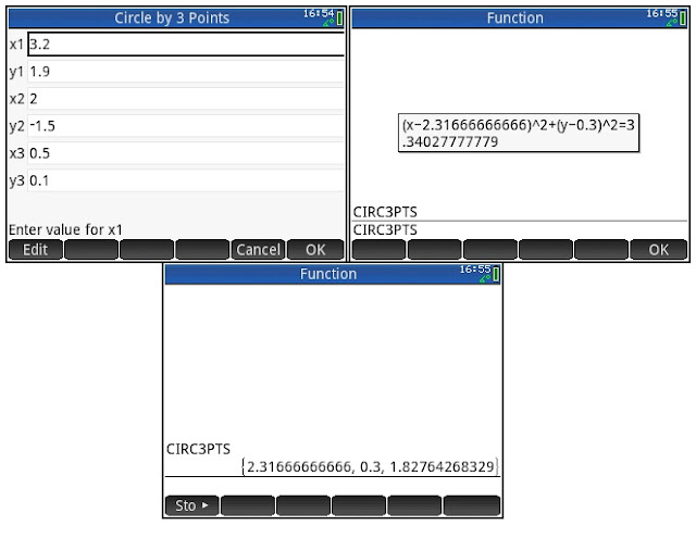
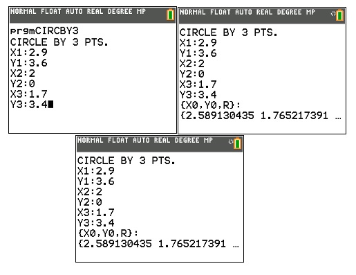
The programs CIRC3PTS (HP Prime) and CIRCBY3 (TI-84 Plus CE) calculate the center and radius of a circle given three points (x1, y1), (x2, y2), and (x3, y3).  The HP Prime will display the equation (x-x0)^2 + (y-y0)^2 = r^2 in a message box.  Both versions will return a list {x0, y0, r}.

The center point (x0, y0) is calculated by:

[ [ x0 ] [ y0 ] ]  =

[ [ x1 – x3, y1 – y3 ] [ x1 – x2, y1 – y2 ] ]^-1 * [ [ a ] [ b ] ]

Where:

a = 0.5 * ( (x1 – x3)*(x1 + x3) + (y1 – y3)*(y1 + y3) )

b = 0.5 * ( (x1 – x2)*(x1 + x2) + (y1 – y2)*(y1 + y2) )

r = √( (x1 – x0)^2 + (y1 – y0)^2 )

HP Prime Program:  CIRC3PTS

EXPORT CIRC3PTS()

BEGIN

// 2016-10-09

// Circle by 3 Points

LOCAL x1,y1,x2,y2;

LOCAL x3,y3,x0,y0;

LOCAL a,b,m,r;

LOCAL str;

// Input box

INPUT({x1,y1,x2,y2,x3,y3},

"Circle by 3 Points",

{"x1","y1","x2","y2",

"x3","y3"});

// Calculation

a:=0.5*((x1-x3)*(x1+x3)+

(y1-y3)*(y1+y3));

b:=0.5*((x1-x2)*(x1+x2)+

(y1-y2)*(y1+y2));

m:=[[x1-x3,y1-y3],[x1-x2,y1-y2]]^-1

*[[a],[b]];

x0:=m(1,1); y0:=m(2,1);

r:=(x1-x0)^2+(y1-y0)^2;

// build string

str:="(x-"+x0+")^2+(y-"+y0+

")^2="+r;

MSGBOX(str);

RETURN {x0,y0,√r};

END;

TI-84 Plus Program:  CIRCBY3

Disp "CIRCLE BY 3 PTS."

Input "X1:",D

Input "Y1:",E

Input "X2:",F

Input "Y2:",G

Input "X3:",H

Input "Y3:",I

0.5*((D-H)*(D+H)+(E-I)*(E+I))→A

0.5*((D-F)*(D+F)+(E-G)*(E+G))→B

[[D-H,E-I][D-F,E-G]]^-1*[[A][B]]→[A]

[A](1,1)→X

[A](2,1)→Y

√((D-X)²+(E-Y)²)→R

Disp "{X0,Y0,R}:"

Pause {X,Y,R}

Test Example:

(x1, y1):  (2, 4)

(x2, y2):  (0, 2)

(x3, y3):  (-1, 3)

Result:

x0 = 0.5

y0 = 3.5

r = 1.58113883008

(x – 0.5)^2 + (y – 3.5)^2 = 2.5

Source:

“Circle Determined by Three Applications” HP-34C Mathematics Applications.  Hewlett Packard, 1979

This blog is property of Edward Shore, 2016.