Showing posts with label math. Show all posts

Saturday, March 15, 2025

Casio Python with fx-CG 50: Drawing Shapes with Casioplot (draws.py)

Casio Python with fx-CG 50: Drawing Shapes with Casioplot (draws.py)


The Casio file draws.py is a file that use both the casioplot and math modules and contains four drawing functions.


The plot functions uses the pixel system.


Upper left hand corner: (0, 0)

Upper right hand corner: (383, 0)

Lower left hand corner: (0, 191)

Lower right hand corner: (383, 191)


The x axis increases going right and the y axis increases going down. This orientation is common for a pixel-orientated coordinate system.


Note that the pixels must be integers. A non-integer value for a pixel will cause an error.


Importing the draws module


After copying the file draws.py to your calculator, type: from draws import *


The casioplot and math modules will also be imported because the draws module is imported. This is the case of the fx-CG 50, and I’m pretty sure it will work with the other Casio calculators with Python (fx-9750GIII, fx-9860GIII, fx-CG 100, Graph Math+).


To clear the drawing screen, use the casioplot’s command clear_screen().


To show the picture, use the casioplot’s command show_screen().


The functions from the draws must be manually typed, as they will not appear in the catalog or VARS menu.


sline(x,sx,y,sy,l,c)


Draws a line from (x,y) of length l and color c. The color is a three-element tuple in the RGB format ((red, green, blue)).


The arguments sx and sy are direction/slope arguments which dictate the direction of the line.


To draw a line going left (←)

Set sx = -1 and sy = 0

To draw a line going right (→)

Set sx = 1 and sy = 0

To draw a line going up (↑)

Set sx = 0 and sy = -1

To draw a line going down (↓)

Set sx = 0 and sy = 1

To draw a line going right and up (↗)

Set sx = 1 and sy = -1

To draw a line going left and up (↖)

Set sx = -1 and sy = -1

To draw a line going right and down (↘)

Set sx = 1 and sy = 1

To draw a line going left and down (↙)

Set sx = -1 and sy = 1


Examples:

sline(1,1,1,0,140,(255,0,0)) draws a red line starting from (1,1) going right with length of 140 pixels


sline(180,0,100,-1,50,(0,255,0)) draws a green line starting from (180,100) going up with length of 50 pixels


The sample file draw1.py is a demonstration of the sline command.


box(x,xl,y,yl,c)


The box function draws a box with the upper left hand corner (x,y) with color c, horizontal length (width) xl, and vertical length (height) yl. The box draws to the right and down. The box is filled with the specified color. If xl = yl, the function will draw a square.


Example:

box(20,100,40,150,(128,128,128)) draws a gray rectangle with upper-left corner at (20,40) with horizontal length of100 and vertical length of 150.


box(300,60,0,60,(0,0,0)) draws a black square with upper-left corner at (300, 0) with the side length of 60.


The sample file draw2.py uses the box function to generate a random game map of land (green) and water (blue).


tri(x,xd,y,yd,l,c)


The tri function draws a 45-45-90 right triangle. The point (x,y) is the corner point that contains the right angle of 90°. The arguments xd and yd dictate the direction of the triangle (see table below).


The triangle is filled with color c. The sides of the triangle will be drawn with length l.


Example:


tri(80,1,80,-1,75,(0,128,128)) draws a teal 45-45-90 right triangle with the right angle located at (80, 80). The length is 75 pixels.


The sample file draw3.py uses the tri function to draw four triangles, one with each proper orientation.


circ(x,y,r,c)


The circ function draws a circle centered at (x, y) with radius r and color c. The circle is drawn as outline and not filled. To make the circle appear as smooth as possible, 720 points are plotted.


Example:

circ(190,100,85,(255,128,0)) draws an orange circle with radius 85, centered at (190, 100).


The file draw4.py demonstrates the circ function.


Casio fx-CG 50 Python: draws.py code


# drawing utilities

# 12-04-2024


from casioplot import *

from math import *


def sline(x,sx,y,sy,l,c):

  for i in range(l+1):

    set_pixel(x+sx*i,y+sy*i,c)


# upper left corner

def box(x,xl,y,yl,c):

  for i in range(xl+1):

    for j in range(yl+1):

      set_pixel(x+i,y+j,c)


# right triangle

# (x,y) point with right angle

# l=length

# xd=1 right, xd=-1 left

# yd=1 down, yd=-1 up

def tri(x,xd,y,yd,l,c):

  for i in range(l+1):

    k=l-i

    for j in range(k+1):

      set_pixel(x+xd*i,y+yd*j,c)


# hallow circle

def circ(x,y,r,c):

for i in range(721):

  t=2*pi*i/720

  xr=int(x+r*cos(t))

  yr=int(y+r*sin(t))

  set_pixel(xr,yr,c)


You can download the draws.py and the example Python files here:

https://drive.google.com/file/d/1rGQHa60V7ZCE9Vs0kYy0cfIe0pOXqVaZ/view?usp=sharing


I hope you enjoy this program as much as I have making it,


Eddie


All original content copyright, © 2011-2025. Edward Shore. Unauthorized use and/or unauthorized distribution for commercial purposes without express and written permission from the author is strictly prohibited. This blog entry may be distributed for noncommercial purposes, provided that full credit is given to the author.

Sunday, June 5, 2022

TI-84 Plus CE Python: Polygon Path (ppath.py)

TI-84 Plus CE Python:  Polygon Path (ppath.py)


Introduction


The program PPATH:


Between two points:  


1.  Calculates the required leftward, counter-clockwise angle.


2.  Calculates the distance to be traveled. 


The path starts at the origin (0,0).  You can create open paths or closed polygons.  For polygons, add another point and include (0,0) as the last point.  


TI-84 Plus CE Python Program:  PPATH - Python (ppath)


Download the TI-84 Plus CE Python file here:  https://drive.google.com/file/d/1QnPP9ikx45i7gAH22fTkFAmE-pBFQwTD/view?usp=sharing


Copy the code for a text file.  


print("Poly Path \nEdward Shore")

# 2022-04-27

from math import *

from turtle import *

t=Turtle()

# t is required for turtle

from ti_system import *


# hide the grid

t.hidegrid()


# obtain the points

x=[0]

y=[0]

# angles

g=[0]

# degree difference

q=[0]

# distance

d=[0]


print("Point 0: (0,0)")

print("#_0 to #_n-1")

n=eval(input("# points? "))


for i in range(1,n):  

  a=eval(input("x"+str(i)+"? "))

  b=eval(input("y"+str(i)+"? "))

  x.append(a)

  y.append(b)

  r=sqrt((a-x[i-1])**2+(b-y[i-1])**2)

  d.append(r)

  m=degrees(atan2(b-y[i-1],a-x[i-1]))

  v=m-g[i-1]

  if v<0:

    v+=360

  g.append(m)

  q.append(v)

  r6=round(r,6)

  m6=round(v,6)

  print("Distance: "+str(r6))

  print("Left Turn: "+str(m6)+"\u00b0")


print("\nPress [clear] to continue.")

disp_wait()


t.home()

t.pencolor(0,128,0)

# set speed

t.speed(4)

for i in range:

  t.left(q[i])

  t.forward(d[i])

t.done()


Notes:


1.  Turtle is a add-in module for the TI-84 Plus CE Python, which must be downloaded. Download the Turtle module here:  https://education.ti.com/en/product-resources/turtle-module/ti84ce-python


2.  Calling the Turtle module automatically assigns the variable t to a drawing turtle by the line t=Turtle().


3.  The ti_system module is exclusive to the TI-84 Plus CE.  This allows the program to pause with the disp_wait command.  


4.  The underscore character ( _ ) can be typed by the [ 2nd ] [ (-) ] (ans) sequence.  


5.  The hashtag character ( # ) can be typed by the [ 2nd ] [ 3 ] (L3) sequence.  


6.  The line for i in range(1,n) starts a for loop with i taking the values from 1 to n-1. This is good for lists when the initial point (point 0) does not need further processing. 


7.  The default operating angle measurement in Python is Radians.  


8.  The angle difference, which tells us how many degrees to turn left, is normalized to the 0°-360° range.   This is optional.   


9.  The line t.home() sets the turtle to point (0,0) and sets the turtle's orientation to 0° (facing right, forward on the x-axis).


10.  The line t.done() shows the results of the turtle commands. 


Examples


Example 1: Quadrilateral


Example 2:  An Open Path


Enjoy!  


Eddie 


All original content copyright, © 2011-2022.  Edward Shore.   Unauthorized use and/or unauthorized distribution for commercial purposes without express and written permission from the author is strictly prohibited.  This blog entry may be distributed for noncommercial purposes, provided that full credit is given to the author. 


Sunday, August 29, 2021

Back to School Reference Sheet

 Back to School Reference Sheet


It's near the end of summer, hence for a lot of students the school year is either about to start or just has started.  


Attached is a link to a quick reference that can be helpful in terms of algebra, pre-algebra, geometry, and trigonometry.  Topics include:


* Solving Equations

* Quadratic Equations

* Completing the Square

* Basic Laws of Logarithms

* Basic Trigonometry Identities

* Some Conversions of Length

* Basic Circle and Right Triangle Properties


I hope you find this useful.   

Good luck, good health, and good fortune to all the students in school this year and may you succeed in all of your studies.

Eddie

All original content copyright, © 2011-2021.  Edward Shore.   Unauthorized use and/or unauthorized distribution for commercial purposes without express and written permission from the author is strictly prohibited.  This blog entry may be distributed for noncommercial purposes, provided that full credit is given to the author. 

Monday, July 19, 2021

Review: TI-84 Plus CE Python

 Review:  TI-84 Plus CE Python


From the looks of the packaging, the CE Python edition is set to replace the non-Python CE.


Python Comes to the TI-84 CE Python

The TI-84 Plus CE Python has started to arrive in the United States.  I was able to purchase a TI-84 Plus CE Python calculator at a local Target (I'm in the greater Los Angeles area).   At the time, Target had three colors:  blue, red, and white.  Since I already have a blue TI-84 Plus CE ("plain", but M hardware revision), I purchased a white calculator.  I was able to get the Python at a price of what the original CE sells for.  Prices vary around $100 to $150, so shop for the back to school sales and discounts.  

The TI-84 Plus CE Python is the TI-84 Plus CE but with the chip added so that the calculator can run Python programs.  You get all the features of the original TI-84 Plus CE, along with all the standard apps (Finance, CabriJr, CelSheet, Conics, PlySmlt2, etc).  However, there is a slight difference in memory:

TI-84 Plus CE:   154,000 bytes RAM, 3MB bytes ROM
TI-84 Plus CE Python:  149,000 bytes RAM, 3MB bytes ROM

It's still plenty of room to work.  

The TI-84 Plus CE Python comes with OS 5.6 installed.  Hence, ASM (assembly) programming is not supported unless a hack is applied to it.  

This review will focus on the Python part, for the rest, please see my review of the original TI-84 Plus CE here, way back in May 2015:

Python


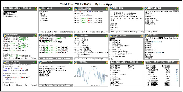
The TI-84 Plus CE Python runs Micropython.  There are several standard modules: math, random, and time, with TI's custom modules:  ti_system, ti_plotlib (graphing), ti_hub (TI Basic programming also gets hub commands), and ti_rover.

I like the menu structure, with most of the commands giving the syntax of each command.   I had a much easier time selecting the commands from the Fns... menu than typing them myself.   For several commands, once they are selected from the Fns... menus, we get a secondary prompt to choose a attribute.  

Examples:  

(1) plt.axes gives a choice of turning them On and Off.   

(2) plt.plot gives a prompt of four possible markers.

Calling commands from Fns... menus pastes the parenthesis and brackets.

Context menus are also available through the [ math ], ( list ), and the trig keys ([ sin ], [ cos ], [ tan ]).  More can be discovered.  In Python, both the [(-)] and [ - ] keys can be used to enter negative numbers.

What is going to take me some time to get used to is the way the [ alpha ] key operates in the Python app.  The [ alpha ] toggles from lower case (default) and upper case.   I can still use the [ 2nd ] [ alpha ] combination to enter alpha-lock but I will also need to use the [ 2nd ] [ alpha ] sequence to exit alpha-lock.  

To either delete or send Python files to archive, press [ 2nd ] [ mem ] [ 2 ] [ alpha ] [ apps ] (B), not listed in the Prgm (program) variables.   Python scripts are counted as App (application) variables (AppVars).  

I find the Python app easy to use.

Below are some sample scripts, which you can download here:

The zip file contains:
LISTDEMO:  demonstration of lists
CMPXARIT:  arithmetic with complex numbers
PLOTFX84:  simple plot of y(x) 

Remember, these are application variables (AppVar Python), not program files.   They are not (as of this blog date) able to be edited on the TI Connect CE software. 

Still Wishing

Still waiting for base conversions, vectors functions (cross, dot, norm, angle between vectors), allowing the days between dates allow for four digit years (the current limits are 1980-2079), complex numbers to be allowed in trigonometric, exponential, and logarithm functions.  Maybe in OS 6.x, fingers crossed, putting it out there in the Universe.  


Eddie

All original content copyright, © 2011-2021.  Edward Shore.   Unauthorized use and/or unauthorized distribution for commercial purposes without express and written permission from the author is strictly prohibited.  This blog entry may be distributed for noncommercial purposes, provided that full credit is given to the author. 


Sunday, October 6, 2019

Fun with the TI-81: Part II

Fun with the TI-81:  Part II

Please check out yesterday's blog entry for Part I.  Now let's continue.

TI-81 Decimal to Fraction:  DECTOFRAC
(148 bytes)

This program converts a number X to fraction as an approximation.  Each successful approximation is displayed until the absolute value of the error falls below 10^-12.  This program is based on a program written for the Radio Shack TRS-80 (see source). 

Variables:
X = Number
H = numerator
I = denominator
Y = error
Used: A, B, C, D, E, F, G, J

Program:
Disp "X="
Input X
IPart X → A
1 → B
X - A → C
0 → D
1 → E
1 → F
0 → G
Lbl 2
A * F + D → H
A * G + E → I
H / I - X → Y
ClrHome
Disp H
Disp "/"
Disp I 
Disp "ERR="
Disp Y
Pause
If abs Y<1e-12 font="">
Stop
C → J
B - A * C → C
J → B
F → D
H → F
G → E 
I → G
Goto 2

Example:
X = 4.7995
4 / 1,  ERR = -.7995
5 / 1,  ERR = .2005
13 / 4, ERR = -.0495
24 / 5,  ERR = 5E-4
1915 / 399, ERR = -1.253133E-6
9599 / 2000, ERR = 0

4.7995 = 9599/2000

Source:

Craig, John Clark  119 Practical Programs for the TRS-80 Pocket Computer  Tabs Books Inc.:  Blue Ridge, PA.  1982 ISBN 0-8306-0061-1 (Paperback)

TI-81 Simple Logistic Regression:  LOGISFIT 
(71 bytes)

The program LOGISFIT fits the statistical data to the equation:

y = 1 / (a + b*e^x)

This program uses the linear regression fit with the following translations:

x' = e^(-x), y' = 1/y

This fit will is good for all data except when y = 0.

Instructions: 
1.  Enter the data through the Stat Edit menu. 
2.  Run LOGISFIT.  The data will be altered. 

Program:
1 → I
Lbl 1
e^( -{x}(I) ) → {x}(I)
{y}(I)⁻¹ → {y}(I)
IS>( I, Dim{x} )
Goto 1
LinReg
Disp "Y=1/(a+be^(X))"
Disp "a"
Disp a
Disp "b"
Disp b

Example:
x1 = 0.5
y1 = 0.384
x2 = 1
y2 = 0.422
x3 = 1.5
y3 = 0.45
x4 = 2
y4 = .468
x5 = 2.5
y5 = .48

Results:
a = 2.001859259
b = .9942654005

Equation:
y = 1 / (2.001859259 + .9942654005*e^x)

Source:

Shore, Edward.  "HP Prime and TI-84 Plus CE: Simple Logistic Regression"  Eddie's Math and Calculator Blog. 2017.  http://edspi31415.blogspot.com/2017/04/hp-prime-and-ti-84-plus-ce-simple.html
Retrieved August 17, 2019

TI -81 Confidence Intervals: INTERVAL
(184 bytes)

The program INTERVAL calculates a confidence interval given the sample's mean (M), variance (V), and number of data points (N).  A Z scored is selected when the user selects one of three confidence levels: 

99%  (0.5% on each side of the curve, Z = 2.575829586)
95%  (2.5% on each side of the curve, Z = 1.959963986)
90%.  (5% on each side of the curve, Z = 1.644853627)

The interval lies between ( M - Z * V/√N,  M + Z * V/√N )

Notes:
1.  Z is used as an control variable and the Z score.
2.  The percent symbol is built of three characters, the degree symbol (°), the forward slash by pressing the [ ÷ ] key (/), the decimal point (.).

Program:
0 → Z
Disp "MEAN="
Input M
Disp "VAR="
Input V
Disp "N="
Input N
Lbl 0
ClrHome
Disp "1. 99°/."
Disp "2. 95°/."
Disp "3. 90°/."
Input P
If P=1
2.575829586 → Z
If P=2
1.959963986 → Z
If P=3
1.644853627 → Z
If Z=0
Goto 0
M + Z * V / √N → U
M - Z * V / √N → V
Disp "INTERVAL"
Disp U
Disp V

Example:
Input:  n = 100, M = 156.39, V = 10.94, 99% confidence interval
Results: 
162.2079576
156.5720424

Source:
Kelly, Kathy A., Robert E. Whitsitt II, M. Deal LaMont, Dr. Ralph A. Olivia, et all.  Scientific Calculator Sourcebook   Texas Instruments Inc.  1981.  (no ISBN number is given)

TI-81 Fresnel Polarization:  MICROPOL
(120 bytes)

Given a microwave transferring from one medium to another with the initial angle with respect to the plane surface that separates the mediums, the following are calculated:

1.  Angle of refraction, θt
2.  Fresnel Horizontal Polarization, R_H
3.  Fresnel Vertical Polarization, R_V

The Law of Refraction:
n1 sin θi = n2 sin θt

Fresnel Horizontal Polarization:
R_H = sin(θ_i - θ_t) / sin(θ_i + θ_t)

Fresnel Vertical Polarization:
R_V = tan(θ_i - θ_t) / tan(θ_i + θ_t)

Variables:
N = n_1  (index of refraction of medium 1)
M = n_2  (index of refraction of medium 2)
θ = θ_i  (angle of incidence)
Z = θ_t (angle of refraction)
H = R_H (Fresnel horizontal polarization)
V = R_V (Fresnel vertical polarization)

Note:  Angles are in degrees

Program:
Deg
Disp "N1="
Input N
Disp "θ="
Input θ
Disp "N2="
Input M
sin⁻¹ (Nsin θ / M) → Z
sin(θ-Z) / sin(θ+Z) → H 
tan (θ-Z) / tan (θ+Z) → V
Disp "REFRACT θ=" 
Disp Z
Disp "H-POLAR="
Disp H
Disp "V-POLAR="
Disp V

Example:
Inputs:  N1 = 1.001, θ = 40°, N2 = 1.333
Results:
REFRACT θ = 28.86146514°
H-POLAR = .2071186671
V-POLAR = .0761259908

Source:
Barue, Geraud  Microwave Engineering:  Land & Space Communications  John Wiley & Sons: Hoboken, NJ 2008.  ISBN 978-0-470-08996-5

TI-81 Hyperbolic Circles: Circumference and Area:  HYPCIRCL
(61 bytes)

The program HYPCIRCL calculates the circumference and area of a circle in hyperbolic space.  Note that this not the same as (normal, regular, everyday) circles in Euclidean space. 

Circumference of a hyperbolic circle: C = 2 π sinh(R)

Area of a hyperbolic circle:  A = 4 Ï€ sinh(R/2)^2

Program:
Disp "HYP CIRCLE"
Disp "R="
Input R
2Ï€ sinh R → C
4 Ï€ (sinh(R/2))² → A
Disp "C="
Disp C
Disp "A="
Disp A

Example:
Input: R = 3
Results: 
C = 62.94416455
A = 56.97380062

Source:
Series, Caroline  "Hyperbolic Geometry MA 448"  2010. Edited Jan. 4, 2013

Eddie

All original content copyright, © 2011-2019.  Edward Shore.   Unauthorized use and/or unauthorized distribution for commercial purposes without express and written permission from the author is strictly prohibited.  This blog entry may be distributed for noncommercial purposes, provided that full credit is given to the author.

Saturday, October 5, 2019

Fun with the TI-81: Part I

Fun with the TI-81:  Part I

Before there there was the TI-82, TI-83 and its family, and the TI-84 Plus and its family, there was the Texas Instrument's original calculator from the 1990, the TI-81!

Translating TI-81 to TI-84 Plus (and Back) 

Most of the commands can be copied directly.  Some caveats to keep in mind:

Disp

The TI-81's Disp (Display command) can only display either a variable's value or a string.  The command can only display one item per line.

The TI-84 Plus' Disp command can list any combination of strings and variable values, separated by a comma.  Each argument will be placed on one line.

Input

The TI-81's Input command can ask for one variable.  There is no prompt string option.  A prompt string will require an extra Disp command.  Also, there is no colon character.

Disp "VAR="
Input A

The TI-84 Plus' Input command can have an optional prompt string.

Input "VAR=", A

Lists 

The TI-81 has two lists that are used for statistical calculations, {x} and {y}.  To recall an element of either {x} or {y}, press [ 2nd ] [ 0 ] or [ 2nd ] [ 1 ], respectively.  The dimensions of the stat lists can be found by pressing [VARS], and selecting Dim{x} under the DIM menu.  Stat lists can't be resized by storing a value to it.

All of the lists for the TI-84 Plus start with a lower case bold "L".  Lists 1-6 can be pressed by [ 2nd ] [ 1 ] through [ 6 ].  There are many lists commands and functions for the TI-84 Plus.

Linear Regression Options

Running linear regression is the LinReg command on the TI-81.  The equation will always be a + bx.

Running linear regression for the TI-84 Plus will need you to designate the x-list and y-list.  There are also various options: a + bx, ax + b, or Med-Med

The If Command and Loops

The TI-81 only has a singular If command, no Then or Else.  The syntax is:

If condition
do if condition is true
skip to here if condition is false

Loops will require the extensive use of Lbl (label), Goto, DS<(, and IS>(.   Lbl and Goto are self-explanatory. 

DS<(var, target).   The value of var is decreased by 1.  The next command is skipped when value < target.

IS>(var, target).  The value of var is increased by 1.  The next command is skipped when value > target. 

In addition to If (which can still do the two-line structure), Lbl, Goto, DS<(, and IS>(, the TI-84 Plus has Then, Else, For, While, and Repeat.

The STO> Button

The TI-81 turns on the ALPHA keyboard when pressing [STO>].

The TI-84 Plus doesn't.

On to the programming...

TI-81 Decimal to Binary Conversion:  BINTODEC
(75 bytes)

Input the binary integer at the prompt.  Use only 1s and 0s. 

Variables:
B = binary representation
D = decimal representation
N, M:  used

Program:
Disp "BIN>DEC"
Input B
0 → D
0 → N
B → M
Lbl 0
2^N * 10 * FPart(M/10) + D → D
IPart(M/10) → M
IS>(N, IPart(log B) + 1)
Goto 0
Disp D

Example:
Input:  B:  1001010
Result:  D:  74

TI-81 Binary to Decimal Conversion:  DECTOBIN
(99 bytes)

Input the decimal integer at the prompt.  The integer needs to be in between 1 and 1024.  Only positive integers are allowed.

Variables:
B = binary representation
D = decimal representation
N, M:  used

Program:
Disp "DEC>BIN"
Disp "1≤D≤1024"
Input D
0 → B
D → M
IPart( log D / log 2 ) → N
Lbl 2
If 2^N ≤ M
B + 1 → B
If 2^N ≤ M
M - 2^N → M
If N ≠ 0 
10 * B → B
DS<(N, 0)
Goto 2
Disp B

Example:
Input:  D:  516
Result:  B:  1000000100

TI-81 Roots of a Quadratic Equation:  QUADEQN
(121 bytes)

This program solves the equation A*X^2 + B*X + C = 0, which allows for real or complex roots.

Variables:
A, B, C:  coefficients
X, Y:  roots

If the discriminant is zero or positive, the roots are real, and are stored in X and Y.

If the discriminant is negative, we have complex roots in the form of X ± Yi, X is the real part, Y is the imaginary part.

Program:
Disp "AX²+BX+C=0"
Input A
Input B
Input C
-B / (2A) → X
(B² - 4AC) / (4A²) → Y
If Y<0 font="">
Goto 0
√Y → Y
X + Y → Y
2X - Y → X
Disp "ROOTS"
Goto 2
Lbl 0
√(abs Y) → Y
Disp "X+YI, X-YI"
Lbl 2
Disp X
Disp Y

Examples:

x^2 + 4x + 5 = 0,  Roots:  2 ± i
Input:  A: 1, B: 4, C: 5
Results:  "X+YI, X-YI", X: -2, Y: 1

x^2 + 5x + 4 = 0,  Roots:  -4, -1
Input:  A: 1, B: 5, C: 1
Results: "ROOTS", X: -4, Y: -1

Tomorrow will be Part 2. Until then,

Eddie

All original content copyright, © 2011-2019.  Edward Shore.   Unauthorized use and/or unauthorized distribution for commercial purposes without express and written permission from the author is strictly prohibited.  This blog entry may be distributed for noncommercial purposes, provided that full credit is given to the author.

Saturday, August 17, 2019

HP Prime and HP 41C/DM 41L: Sum of Two Squares

HP Prime and HP 41C/DM 41L:  Sum of Two Squares 

Introduction

Given a positive integer n, can we find two non-negative integers x and y such that:

n = x^2 + y^2

(x and y can be 0, n is assumed to be greater than 0)


There are several theorems and lemmas that are connected to this famous problem.  As a point of interest, I will briefly describe them here. 

1.  n does not have a representation (n can't be written as x^2 + y^2) if any of n's prime factors is congruent to 3 mod 4 and is raised to an odd power.

2.  If n has a representation, then for an integer k, k^2*n also has a representation.

3.  If n is prime and congruent to 1 mod 4, then n has a representation.  (n has the form of n = 4w + 1 for some non-negative integer w).

The program presented here is the use of iterations to find all possible pairs which fit n = x^2 + y^2.   Some integers do not have representations, others have more than one.  The program will show all possible combinations. 

HP Prime Program SUM2SQ

EXPORT SUM2SQ(n)
BEGIN
// EWS 2019-07-21
// breaking n into a sum of 2 squares
LOCAL r,j,k,l;
// we can more than 1 representation
r:=IP((n/2)^0.5);
l:={};
FOR j FROM 0 TO r DO
k:=(n-j^2)^0.5;
IF FP(k)==0 THEN
l:=CONCAT(l,
{STRING(j)+"^2 + "+
STRING(k)+"^2 = "+
STRING(n)});
END;
END;

RETURN l;
END;


HP 41C/DM 41L Program SUMSQRS

Registers  used:
R00 = n
R01 = counter
R02 = temporary

01 LBL T^SUMSQRS
02 FIX 0
03 STO 00
04  2
05  /
06  SQRT
07  INT
08  1000
09  /
10  STO 01
11  LBL 00
12  RCL 00
13  RCL 01
14  INT
15  X↑2
16  -
17  SQRT
18  STO 02
19  FRC
20  X=0?
21  GTO 01
22 GTO 02
23 LBL 01
24 RCL 01
25 INT
26 T^X = 
27 ARCL X
28  AVIEW
29  STOP
30  RCL 02
31  T^Y = 
32 ARCL X
33 AVIEW
34 STOP
35 LBL 02
36  ISG 01
37  GTO 00
38  T^END
39  VIEW
40  FIX 4
41  RTN

Examples

Example 1:  n = 325
325 = 1^2 + 18^2
325 = 6^2 + 17^2
325 = 10^2 + 15^2


Example 2:  n = 530
530 = 1^2 + 23^2
530 = 13^2 + 19^2

Source:

Dudley, Underwood.  "Elementary Number Theory"  2nd Ed. Dover Publications: New York.  1978. ISBN 978-0-486-46931-7

All original content copyright, © 2011-2019.  Edward Shore.   Unauthorized use and/or unauthorized distribution for commercial purposes without express and written permission from the author is strictly prohibited.  This blog entry may be distributed for noncommercial purposes, provided that full credit is given to the author.

Monday, August 12, 2019

TI-84 Plus CE: Rectangular Waveguide - Cutoff Frequency

TI-84 Plus CE:  Rectangular Waveguide - Cutoff Frequency 

Introduction


The program WAVEGDE computes the cutoff frequency of a rectangular guide.  The waveguide has energy propagating in the TE_m,n mode with dimensions a x b (in meters) with relative permittivity E.  The cutoff frequencies is calculated as:

V = speed of light / √E
where speed of light = 299,792,458 m/s

Cutoff frequency (in Hz):
f_c = V/2 * √( (m/a)^2 + (n/b)^2 )

The second part of the calculation will depend on the target frequency, either the attenuation or phase and group velocities will be calculated:

If f < f_c, attenuation (in nerpers) is calculated:

attenuation = (2 Ï€ f_c)/V * √( 1 - (f/f_c)^2 )

If f > f_c, the phase and group velocities are calculated:

phase velocity = V / √( 1 - (f_c/f)^2 )

group velocity = V * √(1 - (f_c/f)^2 )

TI-84 Plus CE Program WAVEGDE

"EWS 2019-07-14"
Disp "RECTANGULAR WAVEGUIDE"
Input "WIDE (M): ",A
Input "NARROW (M): ",B
Input "PERMITTIVITY: ",E
Disp "HALF-WAVE VARIATIONS", "T-M,N"
Input "M: ",M
Input "N: ",N
Input "FREQUENCY (HZ):",F
299792458/√(E)→V
V/2*√((M/A)²+(N/B)²)→C
Disp "CUTOFF FREQ: (HZ)",C
Pause 
If F
Then
(2Ï€C)/V*√(1-(F/C)²)→U
Disp "ATTENUATION:",U,"NEPERS"
Else
V/√(1-(C/F)²)→P
V*√(1-(C/F)²)→G
Disp "PHASE VELOCITY: M/S",P
Disp "GROUP VELOCITY: M/S",G
End

Examples

Example 1:
A rectangular waveguide has the dimensions 2.7 cm x 1.09 cm with permittivity of 1.    (a = 2.7/100, b = 1.09/100, E = 1).  The waves propagate in the TE_2,1 mode  (m = 2, n = 1).  The target frequency is 10 GHZ (10E9 Hz).

Results:
Cutoff Frequency = 1.767490017E10 Hz
Attenuation = 305.4488993 nepers

Example 2: 
Same as Example 1, but set target frequency as 20 GHZ.

Results:
Cutoff Frequency = 1.767490017E10 Hz
Phase Velocity = 640,624,938.6 m/s
Group Velocity = 140,293,504.8 m/s

Source:

"Rectangular Waveguide Calculations"  HP-65 E.E. Pac 2  Hewlett Packard  Cupertino, CA  1977

Eddie

All original content copyright, © 2011-2019.  Edward Shore.   Unauthorized use and/or unauthorized distribution for commercial purposes without express and written permission from the author is strictly prohibited.  This blog entry may be distributed for noncommercial purposes, provided that full credit is given to the author.

Basic vs. Python: Circle Inscribed in Circle [HP 71B, Casio fx-CG 100]

Basic vs. Python: Circle Inscribed in Circle Calculators Used: Basic: HP 71B Python: Casio fx-CG 100 Introduction ...