Numworks: Polynomial Fit with Numpy (Software version 21 or later)

Numworks:  Polynomial Fit with Numpy  (Software version 21 or later)

The scripts polyfit.py and polyfitg.py perfectly fit a polynomial to a set of points.  For a set of n points, a polynomial of degree n-1 can be perfect fit to the set of points.   For instance,  2 points fit a perfect line,  3 points fit a quadratic polynomial, and 4 points fit a cubic polynomial.    Software version 21 or later is required as the numpy module is used.  

Numworks:  polyfit

polyfit.py:    Fit a number of points to a curve using the numpy module

403 bytes

from math import *

import numpy as np

# 2023-09-25 EWS

n=input("number of points? ")

n=int(n)

d=n-1

x=np.ones(n)

y=np.ones(n)

k=0

while k<n:

  print("point "+str(k+1))

  x[k]=float(input("x? "))

  y[k]=float(input("y? "))

  k+=1

p=np.polyfit(x,y,d)

# list coefficients

print("polynomial vector:")

print("x**n:  coef")

for k in range(n):

  print(str(n-k-1),":  ",str(p[k]))

print(p)

Numworks:  polyfitg

polyfitg.py:   Same as polyfit except a graph of the polynomial is drawn.   The coefficients are shown for 3 before the graph is drawn.  

743 bytes 

from math import *

from time import *

from matplotlib.pyplot import *

import numpy as np

# 2023-09-25 EWS

n=input("number of points? ")

n=int(n)

d=n-1

x=np.ones(n)

y=np.ones(n)

k=0

while k<n:

  print("point "+str(k+1))

  x[k]=float(input("x? "))

  y[k]=float(input("y? "))

  k+=1

p=np.polyfit(x,y,d)

# list coefficients

print("polynomial vector:")

print("x**n:  coef")

for k in range(n):

  print(str(n-k-1),":  ",str(p[k]))

print("\nplotting...")

sleep(3)

# graphing portion

c=(np.max(x)-np.min(x))/100

xc=[]

yc=[]

for i in range(101):

  xp=np.min(x)+i*c

  yp=np.polyval(p,xp)

  xc.append(xp)

  yc.append(yp)

axis((min(xc)-.5,max(xc)+.5,min(yc)-.5,max(yc)+.5)) 

axis(True)

grid(True)

plot(xc,yc,color="purple")

show()

Eddie

All original content copyright, © 2011-2023.  Edward Shore.   Unauthorized use and/or unauthorized distribution for commercial purposes without express and written permission from the author is strictly prohibited.  This blog entry may be distributed for noncommercial purposes, provided that full credit is given to the author. 

Carnival of Mathematics # 216

Carnival of Mathematics # 216

Welcome to a special edition of Eddie's Math and Calculator Blog.  I am once again happy to host the Carnival of Mathematics, which this is the 216th Edition.  The Carnival of Mathematics is facilitated by The Aperiodical.   

Check out the monthly series, where you can also submit articles for future carnival articles, at https://aperiodical.com/carnival-of-mathematics/.

May 2023's Carnival was hosted by Cassandra from Cassandra Lee Yieng's Blog:  https://leeyieng.wordpress.com/2023/05/01/carnival-of-mathematics-215-april-2023/

July 2023's Carnival will be hosted by Vaibhav at Double Root.  Double Root's blog:  https://doubleroot.in/

Gratitude to Ioanna Georgiou for the invitation to host once again.    

The Number 216

In a regular, non-leap year, the 216th day of the calendar is August 4.  On leap years, the 216th day is August 3. 

The digital root of 216 is 9.  (2 + 1 + 6 = 9).

The prime factorization of 216 is 2^3 * 3^3.   Note that 216 = 6^3.  

The divisors of 216 are:  1, 2, 3, 4, 6, 8, 9, 12, 18, 24, 27, 36, 54, 72, 108, and 216.  The sum of the proper divisors are 384, making 216 an abundant number.  

216 hours is 9 days exactly.

216 can be expressed as sums and differences of powers, including:

216 = 3^5 - 3^3

216 = 2 * 10^2 + 4^2

216 = 12^2 + 9^2 - 3^2

216 = 4^4 - (6^2 + 2^2)

216 = 8^3 - (14^2 + 10^2)

The Carnival

Thank you to everyone who submitted an article.  You can submit entries at https://aperiodical.com/carnival-of-mathematics/.

SineRider 

This is a really cool game about mathematics.  The goal is to set a curve so that the snow-people successfully pass through a designated number of gates.  At first, the curves are linear but they get more challenging as the game goes on.  The game also saves your progress. (Screen shots are from the game.)

View Hack Club's intro video on Youtube:  https://www.youtube.com/watch?v=35nDYoIwiA8

Play the game here:  https://sinerider.com/

The Game of Hex:  Submitted by Massimo Dacasto

The game of Hex has two players.  The goal is to connect a string of hexagons from one side to the opposite side.  Each player claims a hexagon with their own color, such as red and blue.  The game of Hex is featured in the 1980s game show Blockbusters.  

The web page Hall of Hexagons is a gallery of moves a player can make to guarantee themselves a connection over a set number of rows.  Check out the gallery here:  https://www.drking.org.uk/hexagons/hex/templates.html.

Peirce's Law:  Jon Awbrey of the Inquiry Into Inquiry blog

This article explains Pierce's Law and provides the proof of the law.  The proof is provided in two ways:  by reason and graphically.  Simply put, for propositions P and Q, the law states:

P must be true if there exists Q such that the statement "if P then Q" is true.  In symbols:

(( P ⇒ Q) ⇒ P) ⇒ P

Article:  https://inquiryintoinquiry.com/2008/10/06/peirces-law/

The law is an interesting tongue twister to say the least.

Praeclarum Theorema:  Jon Awbrey of the Inquiry Into Inquiry blog

Jon Awbrey provides an explanation and proof of the Praeclarum Theorema, also known as the Splendid Theorem, which states:

For statements a, b, c, and d:  

((a ⇒ b) ^ (d ⇒ c)) ⇒ ((a ^ d) ⇒ (b ^ c))

Article:  https://inquiryintoinquiry.com/2008/10/05/praeclarum-theorema/

A Spiral on the Brighton Seafront:  Sam Hartburn

The place is the Brighton Seafront in Brighton, UK.  On the sea front there is a spiral of poles, which is the ratio of radii of the large circle to small circle is about the Golden Ratio ( (1 + √5) ÷ 2 ).   

See this spiral here:  https://samhartburn.co.uk/sh/maths-tourism-a-spiral-on-brighton-seafront/

Green's Windmill & Science Centre

In another travel related article, Tom, an Education Officer and blog writer of mathematics and astronomy, reviews the Green's Windmill and Science Centre in Nottingham, UK.  By the picture posted on Tom's post, this is a place I would like to visit one day.   Tom praises the Windmill for giving vision to the mathematics behind windmills, including displaying an integral equation related to electricity and magnetism:  

∫ dσ V dU/dw + ∫ dx dy dx V δU = ∫ dδ U dV/dw + ∫ dx dy dz U δV

The blog entry also features the work of George Green, a British mathematician.   

Tom's Blog Entry:  https://tommaths.blogspot.com/2023/05/greens-windmill-science-centre-museum.html

Green's Mill and Science Centre's Web Site:  https://tommaths.blogspot.com/2023/05/greens-windmill-science-centre-museum.html

Golden Integration:  John D. Cook

Speaking of the Golden Ratio, John d. Cook demonstrates Monte Carlo integration but instead of using a purely random sequence, a pseudo-random sequence using the fractional values of n * φ, where φ = ( (1 + √5) ÷ 2 ).  The method is demonstrated using Python.

Article:  https://www.johndcook.com/blog/2023/04/29/golden-integration/

Monte Carlo integration has an advantage of ease of calculation, with a cost of having to sample a large amount of points to get an accurate answer.  

A Plan to Address the World Challenges With Math:  Kevin Harnett of Quanta Magazine

The article is an interview with mathematician Minhyong Kim, Director of the International Centre of Mathematical Sciences (ICMS) in Edinburgh, Scotland.  The goal is ICMS is to focus mathematics with humanitarian studies. 

In the article, Kim emphasizes that young mathematicians want to work in diverse fields outside the traditional subjects.  

Article:  https://www.quantamagazine.org/a-plan-to-address-the-worlds-challenges-with-math-20230511/

Web page for ICMS:  https://www.icms.org.uk/

The ICMS's web page for The Mathematics for Humanity program, which has recently launched:  https://www.icms.org.uk/funding-opportunities/mathematics-humanity

Hamilton's Quaternions, or, The Trouble with Triples:  Article by James Propp

Math with a romantic story between William Rowan Hamilton and Catherine Barlow.  Hamilton's infatuation for Barlow lasted, despite the fact that Barlow was married to another man.   Barlow's son needed a tutor in mathematics, and Hamilton was the man to call.  While Hamilton was tutoring her son, he and Barlow discussed Barlow's unhappy marriage.   

Propp then details who Hamilton and Barlow first met, along with the math of quaternions in detail.  

A quaternion is defined an extended complex number represented in the form

q1 * i + q2 * j + q3 * k + q4, with q1, q2, q3, and q4 are real numbers.

When multiplying quaternions the following rules are observed:

i^2 = j^2 = k^2 = -1

i * j = k,   j * i = -k

j * k = i,   k * j = -i

k * i = j,   i * k = -j

The article:  https://mathenchant.wordpress.com/2023/05/17/hamiltons-quaternions-or-the-trouble-with-triples/

Degree of ζ(3)

Here is a stack exchange talking about the integral representation of ζ(3)  (Riemann Zeta function of 3).  As of June 2, 2023, the post has the option question regarding a degree of a group of permutations.   

The open question:  https://math.stackexchange.com/questions/4703662/degree-of-zeta3-as-a-period

I would like to thank everyone who submitted articles for the Carnival of Mathematics.  Gratitude to the Aperiodical for having me as this month's host.   

Eddie 

All original content copyright, © 2011-2023.  Edward Shore.   Unauthorized use and/or unauthorized distribution for commercial purposes without express and written permission from the author is strictly prohibited.  This blog entry may be distributed for noncommercial purposes, provided that full credit is given to the author. 

HP Prime: Edge Diffraction Parametric Plot

HP Prime:  Edge Diffraction Parametric Plot

Introduction

The program EDGEDIFFRAC plots the complex amplitude of edge diffraction.  The equation is:

φp = φ0 / √2 * ( CS(t) + 1/2 * (1 + i) )

where:

φp = complex amplitude 

φ0 = unobstructed amplitude, can be a complex number

CS(t) = Cornu Spiral, defined as CS(t) = C(t) + i * S(t)

Cosine Fresnel Integral

C(t) = ∫( cos (π * s^2 / 2) ds for s = 0 to t)

Sine Fresnel Integral

S(t) = ∫( sin (π * s^2 / 2) ds for s = 0 to t)

i = √-1

HP Prime Program:   EDGEDIFFRAC

Notes:

1.  This program runs in the Parametric app.

2.  To allow for the program to be run from any app, the STARTAPP command is placed in the beginning of the program.

3.  To allow editing in any app, the Parametric. prefix is added to the variables Tmin, Tmax, and Tstep.   

4.  The QUOTE command is used to store functions to the graphing variables X1 and Y1.  

5.  The program runs faster in the emulator than the hardware calculator.  

6.  x1(t) is the real part of φp, and y1(t) is the imaginary part of φp. 

Code:

EXPORT EDGEDIFFRAC()

BEGIN

// Edge Diffraction 

// 2023-02-19 EWS

STARTAPP("Parametric");

// set radians mode

HAngle:=0;

// local variables

LOCAL ch,l,lc,pc;

LOCAL y,λ,z,w,φp;

 

// plot application

INPUT(Z0,"Unobstructed Amplitude",

"φ0:");

CHOOSE(l,"Change Color","Red","Indigo",

"Blue","Orange","Green");

lc:={#FF0000h,#400080h,#FFh,

#FFA500h,#C000h};

X1(COLOR):=lc[l];

Parametric.Tmin:=-5;

Parametric.Tmax:=5;

Parametric.Tstep:=0.25;

A:=RE(Z0);

B:=IM(Z0);

X1:=QUOTE(A/√2*(∫(COS(π*S^2/2),S,0,T)+1/2)

-B/√2*(∫(SIN(π*S^2/2),S,0,T)+1/2));

Y1:=QUOTE(A/√2*(∫(SIN(π*S^2/2),S,0,T)+1/2)

+B/√2*(∫(COS(π*S^2/2),S,0,T)+1/2));

CHECK(1);

STARTVIEW(10);

END;

Examples

Example 1:   φ0 =  2 + 6i

Example 2:  φ0 = 2.29

Source

Woan, Graham.  The Cambridge Handbook of Physics Formulas.  Cambridge University Press:  Cambridge, New York.   2003

All original content copyright, © 2011-2023.  Edward Shore.   Unauthorized use and/or unauthorized distribution for commercial purposes without express and written permission from the author is strictly prohibited.  This blog entry may be distributed for noncommercial purposes, provided that full credit is given to the author. 

TI-84 Plus CE: Tracing Polar Equations

TI-84 Plus CE:  Tracing Polar Equations

Traveling Around the Graphs

The programing BLINKING animates a dot around one of four polar equations:

1.  Ellipse

r = b / √(1 - ε^2 * cos^2 θ), where ε = √(a^2 - b^2)/a, a > b

2.  Cardioid

r = a + (1 + cos θ)

3.  3-Leaf Rose

r = a * cos(3 * θ)

4.  Log Spiral

r = a * e^(b * θ)

Notes:

The point alternates through blue (TI-84 Plus CE color 10), green (14), orange (15), and black (12).   The graph itself is light gray (21).  

r1 is the polar equation r1(θ).

Plotting points (not the polar graph) must be in cartesian coordinates (x,y).   

TI-84 Plus CE Program:  BLINKING

"2023-01-15 EWS"

Radian: Polar: FnOff

ZStandard

{10,14,15,12}→L6

Menu("PLOT","ELLIPSE",10,"CARDIOID",11,"3-LEAF ROSE",12,"LOG SPIRAL",13)

Lbl 10

Disp "A≥B"

Prompt A, B

√(A^2-B^2)/A→E

"B/√(1-E^2*cos(θ)^2)"→r1

Goto 20

Lbl 11

Prompt A

"A*(1+cos(θ))"→r1

Goto 20

Lbl 12

Prompt A

"A*cos(3*θ)"→r1

Goto 20

Lbl 13

Disp "A>0, B>0"

Prompt A,B

"A*e^(B*θ)"→r1

Goto 20

Lbl 20

Input "MAX? ",M

Input "NO. STEPS? ",S

M/S→N

FnOn 1

GraphColor(1,21)

0→P: r1(P)→Q

P>Rx(Q,P)→F: P>Ry(Q,P)→G

Pt-On(F,G,1,12)

For(K,1,S)

Wait 0.25

Pt-On(F,G,1,21)

remainder(K,4)+1→C

K*N→P: r1(P)→Q

P>Rx(Q,P)→F: P>Ry(Q,P)→G

Pt-On(F,G,1,L6(C))

End 

Disp "END"

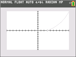
Examples

In all examples, a = 3, b = 2, maximum = 4 * π, steps = 24

Ellipse

Cardioid

 

3-Leaf Rose

Log Spiral

Source

Harris, John W. and Horst Stocker.  Handbook of Mathematics and Computational Science  Springer:  New York.  2006.  ISBN 0-387-94746-9

Eddie

All original content copyright, © 2011-2023.  Edward Shore.   Unauthorized use and/or unauthorized distribution for commercial purposes without express and written permission from the author is strictly prohibited.  This blog entry may be distributed for noncommercial purposes, provided that full credit is given to the author. 

Numworks Software Version 20 Now Available

 Numworks Software Version 20 Now Available 

Click here for details:

https://www.numworks.com/calculator/update/version-20/

Highlights:

*  Separate Finance and Distribution Applications

*  Pressing the divide key [ ÷ ] prior to number entry cycles between:  Ans divided by denominator, fraction, mixed fraction.  

*  Pressing the Home Key then the 0 key gets the shortcut to Settings

*  The new Elements app is available.  We can display each element by its family, s/p/d/f blocks, type of metals, molar mass, electronegativity, melting temperature, boiling temperature, and atomic radius.  Each attribute is shown separately.

* When a value is highlighted in any app, except in Python, pressing [ shift ] (sto→) will give you a prompt to store the amount in a variable.  As a reminder, variables can have more than one character.

*  In the Grapher app, points of interest (zeroes/roots, minima, maxima, points of inflection, etc.) will have black dots.

*  Also in the Grapher app, the ability to find integrals is added to the toolbox.

*  Inverse trig functions are now labeled as arcsin, arccos, and arctan.  

*  Degree and degree minute second templates are loaded from the Toolbox > Units and constants > Length and angle > Angle submenu.

* Additional information is added to angle, trigonometric, and vector calculations.  

* We can add and subtract percents directly.   

There seems to not be additions to the Python programming module (yet).

To update:  just sign in to your Numworks account.  Then connect your calculator, select Update under the Calculator and follow the prompts.  Easy as that!

Thank you, Numworks! 

Eddie

Retro Review: hp 9g

Retro Review:   hp 9g

Quick Facts:

Model:  hp 9g

Company:  Hewlett Packard

Years:  2003 (short production life)

Battery:  2 x AR76 or 2 x LR 44

Display:  10 digits, 2 digit exponent

Logic:  Algebraic - type in expressions the way you write them

Memory:  400 bytes, but can be designated as additional memory registers

Memory Registers:  26, can be extended to 59 memory registers 

Slide Case

Range:  9.999999999 * 10^-99 to 9.999999999 * 10^99, real numbers only

The hp 9g is a small sized graphing calculator, similar to the Citizen SRP-325G and the Casio fx-6300g.  The 9g offers more features than the fx-6300g. 

Features

*  Trig, logs, power, permutations, combinations, hyperbolic functions

*  Random numbers and integers, integer factorials, fraction, integer, sign, absolute value

*  Maximum, minimum, sum, and average up to 10 numbers 

*  Base conversions (decimal, binary, octal, hexadecimal) with Boolean logic (NOT, AND, OR, XOR, NXOR, NEG)

*  20 scientific constants, all SI units   

*  Conversions:  length, area, temperature, volume, mass, calories, pressure (always a good thing to have!)

*  Function graphing, more than one function can be plotted on top of each other.

*  One and Two Variable Statistics

*  Regressions:  linear, logarithmic, exponential, power, inverse, quadratic

Percent

The percent (%) just divides the argument by 100.   For example:  58% converts the number to 0.58.   That is good for multiplying or dividing but not for direct addition and subtraction.

Undo

The [ 2nd ] [ ENTER ] brings back the last thing that has been cleared or deleted.  I don't think this brings back programs that have been deleted though.  

Normal Distribution - One Variable Statistics

Normal distribution is based on one-variable statistics.  The t value is based on data point a_x, which is entered in the DATA menu.  The t point is calculated with the formula:

t = (a_x - mean) / σ

Three areas can be calculated:

P(t):  lower tail cumulative distribution

Q(t):  absolute value of the cumulative distribution between 0 and t

R(t):  upper tail cumulative distribution (I think)

Process Capability - One or Two Variable Statistics

A very unique function, available to the 9G are process capability calculations.  Depending on the mode, the following can be calculated:

C_ax = capability accuracy of x values

C_ay = capability accuracy of y values

C_px = potential precision of x values 

C_py = potential precision of y values

C_pkx = minimum of capability of values or capability precision of x values

C_pky = minimum of capability of values or capability precision of y values

ppm = parts per million (One variable stat mode only)

See the User Manual for formulas.

Storing a Formula

Formulas can be stored into any one of the program areas (P0- P9), using the [ SAVE ] [ PROG ] key sequence.  We can run programs from the Main mode by pressing [ PROG ] with 0 - 9.  Variables are prompted.

Example:  

X^2-3X+1 [ SAVE ] [ PROG ] 9  stores x^2 + 3*x + 1 into program P9.

Evaluating the function at x = -1 and x = 8.5

[ PROG ] 9 [ = ], (formula is displayed), [ = ], [CL/ESC], -1 at the X prompt, [ = ], result:  5

[ PROG ] 9 [ = ], (formula is displayed), [ = ], [CL/ESC], 8.5 at the X prompt, [ = ], result:  47.75

At all prompts, to enter a new number, press [CL/ESC] first, very important.  

Screen

The screen is split up in different sections.  

There are two lines during calculations.  The top line shows what is being calculated, while the bottom line shows the results on the right hand of the screen, in a smaller font.  

In program editing mode, we only get the top line as the bottom of the screen is taken by the two lines EDIT:  and *MAIN* (*DEC/HEX/OCT/BIN* for BASE-N programs).   

In data input, only the top line shows the data points.   

If you graph a function, the left side of the screen is the graph.  Pressing [ Trace ] will alternate between showing the x-coordinate and the y-coordinate.   Personally, I would like it better if both x and y were shown.   The small graph screen means that we really can't do much (no shading, no integration, have to arrow to approximate roots, but can draw lines and plot points).   

Not perfect, but one of the best uses of a small graphics calculator screen.  

Programming

The hp 9g has 400 steps that can be divided among 10 programs (P0 to P9).   Each program can either work in Main mode or Base mode.  Base mode programs are designated for base conversions and Boolean logic.  

The programming language is somewhat like the C programming language.   Each instruction or line can, but doesn't have to end with a semicolon (;).    However, any command called from the INST menu inserts a semicolon.  

Some program commands include:

INPUT var1[, var2, var3... ]  

Input with prompt "[var] = ".  

PRINT "text"/var, "text"/var, ...     

Display strings and variable values

IF (condition) THEN { do if true, commands separated by a semicolon } ; ELSE { do if false, commands separated by a semicolon }

If-Then-Else structure.  The Else part is optional.

Lbl/GOTO n

Lables can take values 0-9

GOSUB PROG n;

Calls a subroutine program n.  Semicolon is required.

SLEEP(time)

Pauses execution for seconds up to 105 seconds.

SWAP(varA, varB)

Swaps the values of variables A and B

; ◢

Stops the program and shows immediate results.   Press [ = ] to continue.

var++, var--   (The ++ and -- is from the INST menu, not pressing + or - twice)

Increase or decrease the variable by 1 after the expression is evaluated.

++var, --var (The ++ and -- is from the INST menu, not pressing + or - twice)

Increase or decrease the varaible by 1 before the epression is evaluated.

FOR(start condition; continue condition; next expression) {loop commands separated by a semicolon}

For loop that works more like a WHILE loop

start condition

WHILE continue condition

loop commands

next expression

END

The FOR loop is in C language.  This is the same syntax of the FOR equation editor command of the Plus42.  

On tomorrow's blog I will have sample programs for the hp 9g.  

Final Thoughts... For Now

I wish the hp 9g had better manuals or manuals that were formatted like a book instead of two large sheets.   But better than nothing and the documentation is detailed.  

The biggest drawbacks are the lack of screen space and small amount of programming steps.  Despite this, the hp 9g is an underrated marvel and is very unique in a line of HP calculators.    

Sources

hp 9g User Manual:  https://literature.hpcalc.org/official/hp9g-ug-en.pdf

hp 9g Examples:  https://literature.hpcalc.org/official/hp9g-htg-en.pdf

"HP 9g"  Wikipedia.   Last edited May 15, 2022.   Last Accessed September 24, 2022.  https://en.wikipedia.org/wiki/HP_9g

 

All original content copyright, © 2011-2022.  Edward Shore.   Unauthorized use and/or unauthorized distribution for commercial purposes without express and written permission from the author is strictly prohibited.  This blog entry may be distributed for noncommercial purposes, provided that full credit is given to the author. 

Python - Lambda Week: Plotting Functions

Python - Lambda Week: Plotting Functions

Welcome to Python Week!  This we we're going to cover calculus and the keyword lambda.

Note:  All Python scripts presented this week were created using a TI-NSpire CX II CAS.   As of June 2022, the lambda keyword is available on all calculators (in the United States) that have Python.   If you are not sure, please check your calculator manual. 

Plotting Functions

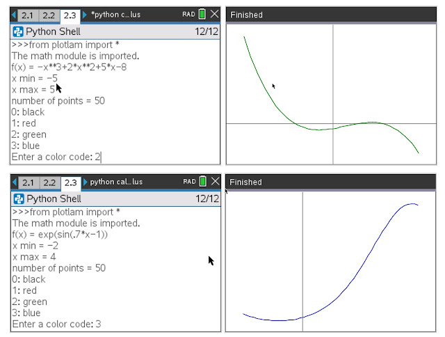
We can use the line:

f=eval("lambda x:"+input("f(x) = "))

for multiple applications.   Remember, lambda functions are not defined so that they can be used outside of the Python script it belongs to but it lambda functions are super useful!

This code is specific to the Texas Instruments calculators (TI-Nspire CX II (CAS), TI-84 Plus CE Python, TI-83 CE Premium Python Edition, but NOT the TI-82 Advanced Python).    For other calculators, HP Prime, Casio fx-CG 50, Casio fx-9750GIII/9860GIII, Numworks, or computer Python, apply similar language. 

plotlam.py:  Plotting with Lambda

from math import *

import ti_plotlib as plt

# this is for the TI calcs

# other calculators will use their own plot syntax

print("The math module is imported.")

# input defaults to string

# use the plus sign to combine strings

f=eval("lambda x:"+input("f(x) = "))

# set up parameters

x0=eval(input("x min = "))

x1=eval(input("x max = "))

# we want n to be an integer

n=int(input("number of points = "))

# calculate step size

h=(x1-x0)/n

# calculate plot lists

x=[]

y=[]

i=x0

while i<=x1:

  x.append(i)

  y.append(f(i))

  i+=h

# choose color (not for Casio fx-9750/9850GIII)

# colors are defined using tuples

colors=((0,0,0),(255,0,0),(0,128,0),(0,0,255))

print("0: black \n1: red \n2: green \n3: blue")

c=int(input("Enter a color code: "))

# plot f(x)

# auto setup to x and y lists

plt.auto_window(x,y)

# plot axes

plt.color(128,128,128)

plt.axes("axes")

# plot the function

plt.color(colors[c])

plt.plot(x,y,".")

plt.show_plot()

All original content copyright, © 2011-2022.  Edward Shore.   Unauthorized use and/or unauthorized distribution for commercial purposes without express and written permission from the author is strictly prohibited.  This blog entry may be distributed for noncommercial purposes, provided that full credit is given to the author. 

Numworks: Version 19.2 Is Available

Numworks:  Version 19.2 Is Available

19.2 Is Here

The full upgrade to software 19.2 is for Numworks N0110 and N0120 models.  Only some of the features will be available for the oldest version N0100. 

How do I know which version I have?  

1.  Press the Yellow Home button.

2.  Go down to Settings and press [ EXE ]

3.  Go down to the last option in the menu, About, and press [ → ]. 

4.  You will see the Software Version.  The last five characters of the FCC ID will tell you what model of Numworks you have.

To update your calculator, just open a browser like Google Chrome, plug in your calculator, go to the numworks.com website.  

Features

Some of the features of 19.2 are (from the Numworks page):

*  The Statistics App now offers four plots: Histogram, Boxplot, Cumulative Frequencies, Normal Probability Plot

*  Median-Median and Exponential regressions are added.

*  Lists are now available everywhere, including the main Calculation app.   List elements are accessed by using the parenthesis (example:  list(1)).  Unlike Python, the first element is designated as element 1.

*  Plots in the Grapher app can be set to any one of seven colors of the user's choosing.

*  Significant tests now include a graphical result in the Inference App

*  The memory for the Python app is increased from 32,000 to 42,000 bytes

*  In the Application menu, each of the apps are assigned to a shortcut key as follows:

1:  Calculation

2:  Grapher

3:  Solver

4:  Statistics (one variable stats)

5:  Regression (two variable stats)

6:  Inference

7:  Sequences

8:  Python

9:  Settings

More information here:  https://www.numworks.com/calculator/update/version-19/

Eddie 

All original content copyright, © 2011-2022.  Edward Shore.   Unauthorized use and/or unauthorized distribution for commercial purposes without express and written permission from the author is strictly prohibited.  This blog entry may be distributed for noncommercial purposes, provided that full credit is given to the author. 

Converting a Line in Parametric Line to a Function Line

Converting a Line in Parametric Line to a Function Line 

From (x(t), y(t)) to y(x)

Express a line, presented in parametric form:

x = A * t + B

y = C * t + D

where A, B, C, and D are constants, and convert it to function form (y(x) or f(x)).

Here is one way to do this:

x = A * t + B

A * t = x - B

t = x / A - B / A

y = C * (x / A - B / A) + D

y = (C/A) * x - B*C/A + D

y = (C/A) * x + (D - B*C/A)

We know have a function in the slope-intercept form where:

slope = C/A

intercept = D - B*C/A

Casio fx-4000P Program:  Converting Parametric Lines to Functional Line

Size:  77 bytes

(line breaks added for readability)

"X=AT+B; A":

?→A:

"B":

?→B:

"Y=CT+D; C":

?→C:

"D":

?→D:

"SLOPE="⊿

C÷A→M⊿

"ITC="⊿

D-B×M→I

Examples

Graph screens are created by the Numworks emulator:  https://www.numworks.com/simulator/

Example 1:

x = 3 * t  - 4 

y = 2 * t + 8

A = 3, B = -4, C = 2, D = 8

Results:

SLOPE = 0.666666667

ITC = 10.66666667

Example 2:

x = -2 * t + 6

y = 4 * t + 3

A = -2, B = 6, C = 4, D = 3

Results:

SLOPE = -2

ITC = 15

Hope you find this useful.  Take care,

Eddie 

All original content copyright, © 2011-2022.  Edward Shore.   Unauthorized use and/or unauthorized distribution for commercial purposes without express and written permission from the author is strictly prohibited.  This blog entry may be distributed for noncommercial purposes, provided that full credit is given to the author.