Sunday, February 25, 2024

Casio Graphing Calculators: Equation Variables

Casio Graphing Calculators: Equation Variables


Introduction


Most modern Casio graphing calculators have an Equation solver mode that solves linear systems (Simultaneous), polynomials (Polynomial), and general equations.


To find run Equation mode, press [ MENU ] { A }*.


(*Equation mode is currently option A (fx-9750GIII, fx-CG 50, fx-CG 10/20, fx-9860 Slim))


Simultaneous Equations: SimRes and SimCoef


The simultaneous equation mode solves linear systems up to 6 x 6. The coefficients of the equations are stored in the variable Sim Coef (labeled SimCoef in VARS-EQUATION menu) while the results are stored in the variable Sim Result (labeled SimRes).


Polynomials: PlyRes and PlyCoef


The polynomial equation mode solves polynomials with real coefficients up to degree 6 (3 in early graphing models). The coefficients of the polynomial are stored in the variable Poly Coef (labeled PolyCoef in the VARS-EQUATION menu) while the results are stored in the variable Poly Result (labeled PolyRes).


Accessing Equation Variables Outside of Equation Mode


The four equation variables can be recalled by pressing [ VARS ], [ F6 ] { > }, [ EQUA ] { F3 }.


F1: SimRes (S·Rlt on older models)

F2: SimCoef (S·Cof on older models)

F3: PlyRes (P·Rlt on older models)

F4: PlyCof (P·Cof on older models)


The four variables are read-only matrices. We can not store values or information to read-only variables.


If we want to extract specific values from the equations variables, we must store them into a Matrix variable (A – Z, θ). For example, to retrieve the number from the 1st row and column of Sim Coef:


Sim Coef → Mat A

Mat A[1,1]


We can execute operations on equation variables. An interesting check is to run the simultaneous solver of the variable by typing:


Rref Sim Coef


and reading the last column.


Until next time,


Eddie


 All original content copyright, © 2011-2024. Edward Shore. Unauthorized use and/or unauthorized distribution for commercial purposes without express and written permission from the author is strictly prohibited. This blog entry may be distributed for noncommercial purposes, provided that full credit is given to the author.


Saturday, February 24, 2024

Swiss Micros DM42 and HP 42S: Moon Landing Simulator from the HP 33-E Applications Book

Swiss Micros DM42 and HP 42S: Moon Landing Simulator from the HP 33-E Applications Book


Landing the Rocket


The goal is to provide enough fuel to get the rocket to land on the moon safely. The use of fuel pushes the rocket away from the surface and slow down the descent. Don’t crash or use too much fuel to escape into space.


Variables:


X: Position

V: Velocity

F: Fuel

G: Gravity

B: Amount of Fuel to burn


Initial Values (from the HP-33E Applications):

X = 500

V = -50

F = 120

G = 5


I wasn't sure about the win condition (X = 0, V = 0?).


I show the position, velocity, and fuel after each successful turn. Enter the amount of units to burn at the burn prompt.


Download here: https://drive.google.com/file/d/1YsYzIMxALuRx_MHSSzGFFEQJdrN656DS/view?usp=sharing


DM42 and HP 42S Code: MOON


00 { 184-Byte Prgm }

01▸LBL "MOON"

02 500

03 STO "X"

04 -50

05 STO "V"

06 120

07 STO "F"

08 5

09 STO "G"

10▸LBL 01

11 "POS:"

12 ARCL "X"

13 AVIEW

14 STOP

15 "VEL:"

16 ARCL "V"

17 AVIEW

18 STOP

19 "FUEL:"

20 ARCL "F"

21 AVIEW

22 STOP

23 RCL "X"

24 X=0?

25 GTO 07

26▸LBL 02

27 "BURN?"

28 PROMPT

29 STO "B"

30 RCL "F"

31 X<Y?

32 GTO 05

33▸LBL 03

34 RCL "B"

35 STO- "F"

36 RCL- "G"

37 STO "A"

38 RCL "V"

39 RCL+ "X"

40 RCL "A"

41 2

42 ÷

43 +

44 STO "X"

45 X≥0?

46 GTO 04

47 GTO 06

48▸LBL 04

49 RCL "V"

50 RCL+ "A"

51 STO "V"

52 GTO 01

53▸LBL 05

54 2

55 RCL× "G"

56 RCL "V"

57 X↑2

58 +

59 SQRT

60 +/-

61 STO "V"

62▸LBL 06

63 "VEL:"

64 ARCL "V"

65 AVIEW

66 "YOU LOSE"

67 AVIEW

68 RTN

69▸LBL 07

70 "SUCCESS!"

71 AVIEW

72 .END.


Example Game


XEQ "MOON"


Initial Turn

POS: 500

VEL: -50

FUEL: 120


BURN? 0

POS: 447.5

VEL: -55

FUEL: 120


BURN? 0

POS: 390

VEL: -60

FUEL: 120


BURN? 0

POS: 327.5

VEL: -65

FUEL: 120


BURN? 5

POS: 262.5

VEL: -65

FUEL: 115


BURN? 0

POS: 195

VEL: -70

FUEL: 115


BURN? 5

POS: 125

VEL: -70

FUEL: 115


BURN? 10

POS: 57.5

VEL: -65

FUEL: 100


BURN? 12.5

"YOU LOSE" -3.75


So close. Good luck!


Source


HP-33 Applications. Hewlett Packard. Corvallis, OR. February 1978


Eddie


All original content copyright, © 2011-2024. Edward Shore. Unauthorized use and/or unauthorized distribution for commercial purposes without express and written permission from the author is strictly prohibited. This blog entry may be distributed for noncommercial purposes, provided that full credit is given to the author.

Sunday, February 18, 2024

Casio fx-CG 50 CORDIC Simulation: Approximating Sine and Cosine of Angles

Casio fx-CG 50 CORDIC Simulation:  Approximating Sine and Cosine of Angles


Introduction - How Computers Calculate Mathematical Functions


First developed by Jack E. Volder, the Coordinate Rotation Digital Computer, better known as CORDIC, is an algorithm used to calculate many mathematical functions, including trigonometric functions, logarithms, exponentials, and hyperbolic functions.     CORDIC is a fundamental algorithm, which variants of CORDIC are used in computers and calculators.


Today's focus will be a calculating sines and cosines of angles.  The steps will be detailed in the next sections.  


CORDIC1:  Series of Arctangents


Let Θ be the angle.   The first step is to build Θ as additions and subtractions of terms of arctan(1 ÷ (2^n)), starting at n = 0 and stopping at the required accuracy.  Let A be the approximation.  


Examples: 


Θ = 45° requires only one term:

A = 45° = arctan 1


Θ ≈ 71.56505118°

 A = 71.56505118° = arctan 1 + arctan 1/2


Θ ≈ 32.47119229°

A = 32.47119229° = arctan 1 - arctan 1/2 + arctan 1/4


A series to recreate Θ = 30° takes 32 terms of ±arctan (1 ÷ 2^n) from n = 0 to n = 31.   (8 decimal places)  This is known as coordinate rotation.


The program CORDIC1 determines the number of terms need to created to obtain Θ.   Accuracy in this code is set to 5 decimal places, but can be adjusted (see the line in blue).  


Casio fx-CG 50 Program Code:  CORDIC1


Deg

"ANGLE"?->Θ

0->I

0->A


Lbl 0

tan^-1 (2^(-I))->T

If A<Θ

Then 

A+T->A

Else 

A-T->A

IfEnd


I+1->I


Abs (A-Θ)>1×10^-5=>Goto 0


ClrText

Blue Locate 1,3,"Θ: "

Blue Locate 5,3,Θ


Red Locate 1,4,"A: "

Red Locate 5,4,A


Green Locate 1,7,I


Notes:

-> is the store arrow →

=> is the jump command ⇒


For reference:


arctan 1 = 45°

arctan 1/2 ≈ 26.56505118°

arctan 1/4 ≈ 14.03624347°

arctan 1/8 ≈ 7.125016349°

arctan 1/16 ≈ 3.576334375°

arctan 1/32 ≈ 1.789910608°


CORDIC2:  Calculating Sine and Cosine


Imagine the coordinate (cos Θ, sin Θ) on a unit circle.  A unit circle is a circle with radius of length 1 and center located at the origin (0,0).   


Set the initial angle at 0°.  Then x = cos 0° = 1 and y = sin 0° = 0.   The initial vector is set to be [ [ cos 0° ] [ sin 0° ] ] = [ [ 1 ] [ 0 ] ].


Approximate Θ in terms of arctangent (1 ÷ (2^n)), starting at n = 0.  


Direction of Rotation


Set σ as the direction of rotation.    


A rotation is positive if we add arctan(1 ÷ (2^n)) to A.    For a positive rotation, set σ_i = +1.   


A rotation is negative if we subtract arctan(1 ÷ (2^n)) to A.    For a negative rotation, set σ_i = -1.   


For example:


 Θ ≈ 32.47119229°

A = 32.47119229° = arctan 1 - arctan 1/2 + arctan 1/4


Then:  σ_0 = 1 (positive rotation), σ_1 = -1 (negative rotation), σ_2 =  1 (positive rotation).  


Multiplying Factor


The number of iterations is also used to determine the required multiplication factor:


n = Π( 1 ÷ √(1 + 2^(-2 × I)), I = 0 to I = terms needed - 1)


For the example:


 Θ ≈ 32.47119229°

Needed 3 iterations, i_0 to i_2.  


Then:

n = 1 ÷ √(1 + 2^(-2 × 0)) × 1 ÷ √(1 + 2^(-2 × 1)) × 1 ÷ √(1 + 2^(-2 × 2))

= 4 × √170 ÷ 85

≈ 0.6135719911


Calculating the Next Iteration


The next iteration for x and y are:


x_i+1 = x_i - 2^(-i) × σ_i × y_i


y_i+1 = 2^(-i) × σ_i × x_i + y_i


When A is sufficiently near or equal to Θ, the cosine and sine are approximated as:


cos(A) ≈ n × x_final


sin(A) ≈ n × y_final


For the example:

 Θ ≈ 32.47119229°


The approximated angle, in this case, happens to be exact angle, A = Θ.  And,

cos(A) ≈ 0.8436614877 

sin(A) ≈ 0.5368754922


For more details, please check out resources in the Sources section.   I particularly like Oxford's A Very Short Introduction series.  


Casio fx-CG 50 Program Code:  CORDIC2


This algorithm is adopted from the Python example (see Wikipedia article).  


Deg

"ANGLE"?->Θ


0->I

0->A

1->X

0->Y

1->N


Lbl 0

tan^-1 (2^(-I))->T

If A<Θ

Then 

A+T->A

1->S

Else 

A-T->A

-1->S

IfEnd

N÷√(1+2^(-2*I))->N

X-S*2^(-I)*Y->P

Y+X*S*2^(-I)->Q

P->X

Q->Y


I+1->I


Abs (A-Θ)>1×10^-5=>Goto 0

X*N->X

Y*N->Y


ClrText

Blue Locate 1,3,"Θ: "

Blue Locate 5,3,Θ


Red Locate 1,4,"A: "

Red Locate 5,4,A


Black Locate 1,5,"cos :"

Black Locate 7,5,X

Black Locate 1,6,"sin :"

Black Locate 7,6,Y


Green Locate 1,7,I


CORDIC3:  Doing it without a Arctangent function


In reality, most of the time the arctangent function also has to be approximated.   There are many ways to approximate, which varying accuracy.   I used the fx-CG50's statistics mode to come up with a regression equation with the following lists:


x_list = sequence of 1÷(2^i) from i = 0 to i = 39 


y_list = sequence of arctan(1÷(2^i)) from i = 0 to i = 39


Of the regression models the fx-CG50 offers, the best regression model is quartic regression (4th-order polynomial):


y ≈ 9.43597784 × x^4 - 22.116232 × x^3 + 0.40116676 × x^2 + 57.2790727 × x + 1.4558 × 10^-5


Remember that I am working with degree angle measurement.  


Casio fx-CG 50 Program Code:  CORDIC3


Deg

"ANGLE"?->Θ


0->I

0->A

1->X

0->Y

1->N


Lbl 0

2^(-I)->K

9.43597784917955K^(4)-22.1162323028173K^(3)+

0.401166766193516K^2+57.2790727477367K+

1.45584715586876×10^-5->T


If A<Θ

Then 

A+T->A

1->S

Else 

A-T->A

-1->S

IfEnd

N÷√(1+2^(-2*I))->N

X-S*2^(-I)*Y->P

Y+X*S*2^(-I)->Q

P->X

Q->Y


I+1->I


Abs (A-Θ)>1×10^-5=>Goto 0

X*N->X

Y*N->Y


ClrText

Blue Locate 1,3,"Θ: "

Blue Locate 5,3,Θ


Red Locate 1,4,"A: "

Red Locate 5,4,A


Black Locate 1,5,"cos :"

Black Locate 7,5,X

Black Locate 1,6,"sin :"

Black Locate 7,6,Y


Green Locate 1,7,I


For the example:

 Θ ≈ 32.47119229°


Approximating Θ within 8 decimal places (10^-5) yields these results:

A:  32.47118598

cos A:  0.8436683456

sin A:  0.5368647154

24 terms used


Sources


"CORDIC"  Wikipedia.   Last Edited January 11, 2024.   Accessed January 12, 2024.  https://en.wikipedia.org/wiki/CORDIC


Brummelen, Glen Van.  Trigonometry:  A Very Short Introduction  Oxford University Press: Oxford, United Kingdom.  2020.  ISBN 978-0-19-881431-3


Eddie


All original content copyright, © 2011-2024.  Edward Shore.   Unauthorized use and/or unauthorized distribution for commercial purposes without express and written permission from the author is strictly prohibited.  This blog entry may be distributed for noncommercial purposes, provided that full credit is given to the author. 


Saturday, February 17, 2024

TI-30Xa Algorithms: Annuity Factors

TI-30Xa Algorithms:   Annuity Factors


Introduction


Even when a calculator isn't (technically) programmable, algorithms can be applied to scientific and financial calculations.


The calculations take numerical arguments that are stored in the TI-30Xa's three memory slots:  M1, M2, and M3.  Store amounts into the memory registers by the [ STO ] key.  


Careful:  For the solar versions of the TI-30Xa, do not press the [ON/AC] button as doing so clears the memory registers.


Today's list of routines deals with annuity factors.


SPFV:  Future Value of a Single Present Value Factor


SPFV = (1 + i%)^n


FV = PV × SPFV


SPPV:  Present Value of a Single Future Value Factor


SPPV = (1 + i%)^(-n)


PV = FV × SPPV


USFV:  Future Value of a Payment Stream Factor


USFV = ((1 + i%)^n - 1) ÷ i%


FV = PMT × USFV


USPV:  Present Value of a Payment Stream Factor


USPV = (1 - (1 + i%)^(-n)) ÷ i%


PV = PMT × USPV


where:

PV = present value

PMT = payment

FV = future value

n = number of periods

i% = periodic interest rate


For monthly payments per year:

n = number of years × 12

i% = annual interest rate ÷ 12


For quarterly payments per year:  

n = number of years × 4

i% = annual interest rate ÷ 4


For the routines, n is stored in memory register 1 and i% is stored in memory register 2. 


n [ STO ] 1 

i% [ STO ] 2


SPFV:  Future Value of a Single Present Value Factor


 [ ( ] 1 [ + ] [ RCL ] 2 [ 2nd ] { % } [ ) ] [ y^x ] [ RCL ] 1 [ = ]


SPPV:  Present Value of a Single Future Value Factor


 [ ( ] 1 [ + ] [ RCL ] 2 [ 2nd ] { % } [ ) ] [ y^x ] [ RCL ] 1 [ ± ] [ = ]


USFV:  Future Value of a Payment Stream Factor


[ ( ] [ ( ] 1 [ + ] [ RCL ] 2 [ 2nd ] { % } [ ) ] [ y^x ] [ RCL ] 1 [ - ] 1 [ ) ] 

[ ÷ ] [ RCL ] 2 [ 2nd ] { % } [ = ]


USPV:  Present Value of a Payment Stream Factor


[ ( ] 1 [ - ] [ ( ] 1 [ + ] [ RCL ] 2 [ 2nd ] { % } [ ) ] [ y^x ] [ RCL ] 1 [ ± ] [ ) ]

[ ÷ ] [ RCL ] 2 [ 2nd ] { % } [ = ]


Example


Let n = 60, i% = 5  


60 [ STO ] 1

5 [ STO ] 2


SPFV:  18.67918589

SPPV:  0.053535524

USFV:  353.5837179

USPV:  18.92928953


Eddie


All original content copyright, © 2011-2024.  Edward Shore.   Unauthorized use and/or unauthorized distribution for commercial purposes without express and written permission from the author is strictly prohibited.  This blog entry may be distributed for noncommercial purposes, provided that full credit is given to the author. 


Sunday, February 11, 2024

Spotlight: Casio CFX-9850GB Plus

Spotlight:   Casio CFX-9850GB Plus 

(Retro Review)


Quick Facts


Model:  CFX-9850GB Plus

Company:  Casio

Timeline:  late 1990s (circa 1997) to 2008

Type:   Graphing, Algebraic, floating decimal with fractions

Number of Digits:  10

Power:  4 AAA batteries plus CR 2032 backup

Colors:  orange, blue, green

Screen Size:  128 x 64 pixels


There are two versions of the CFX-9850GB Plus:  


*  First edition (1997 - 2002):  Black case, black slide cover, about 32,000 bytes of memory.   


*  Second edition (2002 - 2008):  White case, green cover, about 64,000 bytes of memory.


I have the first edition.   Even though this calculator is no longer in production, the CFX-9850G series is still available through online sites such as eBay and thrift stores.  I purchased mine on eBay from Petchiart Shop.  


Graphing in Color


The CFX-9850G series is the first series of calculators to include a multicolored display.   Graphs, tables, statistical plots, and sequences can be displayed in up to three colors:  blue, green, and orange.  


How were the colors accomplished?  Colors are determined by the contrast of the pixels.  Pixels with the lightest contrast are displayed as orange.  Pixels with a medium contrast are displayed as blue.  Pixels with the darkest contrast are displayed as green.  


Text and regular calculations are shown in blue.  We can change the color of the text to green or orange through [OPTN], [F6] (>), [F1] (COLR).   Blue text is the default.  


Calculator Modes


1  Run:  Main Calculator

2  Statistics:  Statistics. Regressions include linear, med-med, quadratic, cubic, quartic, logarithmic, exponential, power, sinusoidal, and logistic.

3  Matrices:  Matrix editing and manipulation mode

4  Lists:  List editing and manipulation mode.  Up to six lists can be stored (List 1 - List 6)

5  Graphing:  Functions with and without shading (Y(X)), Polar (r(Θ)), Parametric (X(T), Y(T)), Horizontal Lines (x=c) 

6  Dynamic Graphing:  Leave one variable to change during graphing

7  Tables

8  Recursion:  graphing recursion sequences

9  Conics:  graphing conics using templates

A  Equation:  Simultaneous linear systems to the order of 6 equations, quadratic polynomials, cubic polynomials, general solver

B  Program:  Programs can be write-protected with a password if desired. 

C  TVM:  Finance including simple interest, compound interest, amortization, cost/sell/margin, date addition, days between dates

D  Link

E  Contrast menu

F  Memory Manager


Also included through the [OPTN] key:


Complex numbers:  arithmetic, parts (real, imaginary, absolute value, argument/angle), conjugate


Hyperbolic functions


Probability functions


Numeric function including fractional and integer parts, rounding function (internally round the number to fix settings).


Angle:  Angle units including decimal degrees/degree-minute-second conversions


Logic:  AND, OR, NOT.   The calculator has integer modes (decimal, octal, hexadecimal, binary).  


Function Memory:  store up to 6 functions for recall.   


ESYM:  engineering suffixes (mega, micro, etc)


The calculator is run in LineIO format (linear).  There is no textbook mode or an exact function when it comes to terms of pi (π) or square roots (√).


Peripherals


To transfer files between the calculator and a computer, the CFX-9850GB Plus uses an FA-123 connection cable.  If this calculator is not purchased new or like new, the cable will have to be a separate purchase, which may not be an easy find.   I believe the FA-123 is a USB cable.   


There is a SB-62 cable which connects the calculator to a class of Casio label printers, such as the Casio KL-2000 Printer.   


Built-In Library


What separates the CFX-9850GB PLUS (and the CFX-9950GB PLUS) from the rest of the series is the inclusion of a built in software library which can be loaded into the calculator's memory at any time.   All of the library's programs are write-protected and require a password to edit.  I don't know the password, sorry.


The software library includes programs that used the EA-100 data analyzer,  differential equations, drawing Mandelbrot sets, geometry, amortization, complex number powers and roots, double and triple integrals, and slope filed graphs.  (not an all-inclusive list).


I want to try them all.


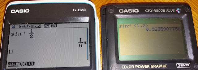
Comparison of the Color Calculators  (vs. fx-CG 50)


I want to close out this spotlight by comparing the CFX-9850 PLUS with its LCD contrast pixels versus the current Casio fx-CG 50, a full-color graphing calculator.  


In the following pictures, the fx-CG50 is on the left, the CFX-9850GB PLUS is on the right. 


Sources


"CFX-9850G PLUS"   Casio Ledudu.  2022.   Accessed January 9, 2024.  https://casio.ledudu.com/pockets.asp?type=280&lg=eng

(this link includes the main manual)


"Casio 9850 series"  Wikipedia.  Last Edited May 14, 2023.  Accessed December 30, 2023.  https://en.wikipedia.org/wiki/Casio_9850_series


Casio.   Casio CFX9850GB Plus Software Library.  https://support.casio.com/en/manual/manualfile.php?cid=004013009

Accessed December 30, 2023. 


Vis, Peter. "Casio Serial Cable Compatibility"   The Quantum Archive.   Accessed January 9, 2024.  https://www.petervis.com/electronics%20guides/Casio%20Serial%20Cables/Casio%20Serial%20Cable%20Compatibility.html


I am always impressed with Casio graphing calculators.   Often, they give the most functions and capability for the least money.  Money well spent.  


Eddie


All original content copyright, © 2011-2024.  Edward Shore.   Unauthorized use and/or unauthorized distribution for commercial purposes without express and written permission from the author is strictly prohibited.  This blog entry may be distributed for noncommercial purposes, provided that full credit is given to the author. 


Saturday, February 10, 2024

Spotlight: Aristo Multilog Nr. 970 Slide Rule

Spotlight: Aristo Multilog Nr. 970 Slide Rule


Release Year:  1954


Santa Barbara and Carpentaria, California, are two of my favorite places to visit.   While on vacation in December 2023 in Santa Barbara, I bought a Aristo Nr. Slide Rule at Antique Alley.  


Not only did the slide rule have a nice, hard case, the slide rule is large. The slide rule also has a functional description of each scale.  I also like the slide rule uses two colors, black and brown, to distinguish the scales from each other.  


Side 1:


LL00:   e^(-0.001X)

K:  X^3  (K = D^3)

A:  X^2  (A = D^2)

CF:  πX  

CIF:  1/(πX)

L:  lg X  (log X)

CI:  1/X

C:  X

D:  X

DI:  1/X

LL0:  e^(0.001X)


Side 2:


LL01:  e^(-0.01X)

LL02:  e^(-0.1X)

LL03:  e^(-X)

DF:  πX

B:  X^2

T:  ∡tg   (tan X, X is in degrees, tan D° = T)

ST:  ∡arc  (tan X, sin X)

S:  ∡sin  (arcsin X, sin D° = T) 

C:  X

D:  X 

LL3:  e^X  (LL3 = e^D)

LL2:  e^(0.1X)

LL1:  e^(0.01X)


As a bonus, the slide rule came with a reference card.  One one side is the Dietzgen Slide Rule Conversion Tables  (U.S. and SI units, 1950), and other side is a table of common areas, surface areas, volumes, and trigonometric properties of the right triangle.   I don't know if this was standard addition when the Aristo Multilog Nr. 970 was sold.  


This may be my favorite slide rule:  not only the scales are large (and as a result easier on the eyes to read), but the fact that there are function descriptions on the scales is a big plus.  


Eddie


All original content copyright, © 2011-2024.  Edward Shore.   Unauthorized use and/or unauthorized distribution for commercial purposes without express and written permission from the author is strictly prohibited.  This blog entry may be distributed for noncommercial purposes, provided that full credit is given to the author. 


BA-54: Real Estate Programs

BA-54: Real Estate Programs BA-54:  Chris won this calculator at HHC 2024 and donated it to me.   Much appreciation as always.  ...