TI-84 Plus CE: Signal to Noise Ratio and Shannon’s Law

TI-84 Plus CE: Signal to Noise Ratio and Shannon’s Law

Signal to Noise Ratio (SNR)

The program SNR calculates the signal to noise ratio for inputs in one of the three units:

Decibels	S – N
Watts	20 * log( S ÷ N )
Voltage	10 * log(S ÷ N )

S: desired signal level

N: noise level

Cadence PCB Solutions (see source) provides a scale of signal to noise ratios and their effectiveness, which is summarized here:

5 dB to 10 dB	No connection is made, the ratio is too low
10 dB to 15 dB	The connection is unreliable
15 dB to 25 dB	Minimum acceptable level
25 dB to 40 dB	Good connection
41 dB and above	Excellent connection

In general, the higher the SNR, the better.

TI-84 TI-Basic Code: Signal to Noise Ratio

Program Title: SNR

Menu(“SIGNAL NOISE RATIO”,”DECIBELS”,1,”WATTS”,2,”VOLTAGE”,3)

Lbl 1

Input “SIGNAL DB? “, S

Input “NOISE DB? “, N

S – N → R

Goto 0

Lbl 2

Input “SIGNAL (W)? “, S

Input “NOISE (W)? “, N

20 * log(S / N) → R

Goto 0

Lbl 3

Input “SIGNAL (V)? “, S

Input “NOISE (W)? “, W

10 * log(S / N) → R

Goto 0

Lbl 0

Disp “SNR (DB): “, R

Examples

Example 1: S: -10 dB, N: -50 dB (from Source)

Results: 40 dB

Example 2: S: 400 W, N: 60 W

Results: 16.47817482 dB

Example 3: S: 300E-3 V (300 millivolts), N: 2E-6 V (2 microvolts)

Result: 51.76091259 dB (*source erroneously had 62 DB)

Shannon’s Law

The program SHANNON makes two calculations: signal to noise ratio in decibels and the capacity of the channel in bits per second. Shannon’s Law was discovered by Claude Shannon during World War II.

C = W * log(1 + S ÷ N) ÷ log(2)

W: bandwidth of the signal in Hertz

S: average signal received in Watts

N: average noise signal in Watts

C: maximum channel capacity in Bits per Second

TI-84 TI-Basic Code: Shannon’s Law

Program Title: SHANNON

Disp “SHANNON’S LAW”

Input “REC’D POWER (W)? “, S

Input “NOISE POWER (W)? “, N

Input “BANDWIDTH (HZ)? “, W

20 * log(S / N) → R

Disp “SIGNAL NOISE RATIO: “, R

W * log(1 + S / N) / log(2) → C

Disp “CHANNEL (BITS/S):”, C

Example

Inputs:

Average Received Signal Power (S): 49.2 W

Average Noise Power (N): 2.2 W

Bandwidth: 200 Hz

Results:

Signal Noise Ratio (SNR): 26.99084844 dB

Channel capacity: 909.2385861 bits/s

Source

Cadence. “What is Signal to Noise Ratio and How to calculate it?” Cadence PCB Solutions. 2020. Accessed November 30, 2025. https://resources.pcb.cadence.com/blog/2020-what-is-signal-to-noise-ratio-and-how-to-calculate-it

Eddie

All original content copyright, © 2011-2026. Edward Shore. Unauthorized use and/or unauthorized distribution for commercial purposes without express and written permission from the author is strictly prohibited. This blog entry may be distributed for noncommercial purposes, provided that full credit is given to the author.

TI-84 Plus CE and DM42: RLC Circuits

TI-84 Plus CE and DM42: RLC Circuits

The program RLC calculates:

(1) The total impedance across the entire circuit

(2) The phase angle, sometimes known as a power factor angle

(3) The total supply current

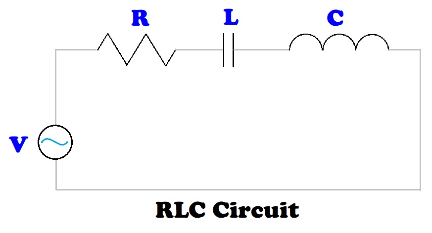
An RLC circuit is a circuit that connects one power supply to a resistor, an inductor, and a capacitor. The resistor, inductor, and capacitor can be connected in one of two ways: series or parallel. To calculate the total impedance (Z) and phase angle (θ), the rectangular to polar conversion function can be utilized.

In a general rectangular to polar conversion, (x, y) to (r, θ):

r = √(x^2 + y^2)

θ = arctan(y / x)

Formulas

Angular Frequency: ω = 2 * π * F	F = frequency in Hz V = supply voltage (volts) R = resistor in Ω (ohms) L = inductor in H (henrys) C = capacitance (farads) I = overall current (amps)
Series RLC Circuit - Formulas Z = √(R^2 + (ω*L – 1 / (ω*C))^2) θ = arctan ( (ω*L – 1 / (ω*C)) / R) I = V / Z	Series RLC Circuit – Set up for Rectangular to Polar Conversion x = ω*L – 1 / (ω*C) y = R Z = r
Parallel RLC Circuit - Formulas 1 / Z = √( (1/R)^2 + (1/(ω*L) – ω*C)^2) θ = arctan ( (1/(ω*L) – ω*C) / (1/R)) I = V / Z	Parallel RLC Circuit – Set up for Rectangular to Polar Conversion x = 1/(ω*L) – ω*C y = 1/R Z = 1/r

TI-84 Plus Program: RLC

ClrHome

Disp “RLC CIRCUIT”

Input “SUPPLY VOLTAGE? “, V

Input “FREQUENCY (HZ)? “, F

Input “RESISTANCE (OHMS)? “, R

Input “INDUCTOR (HENRYS)? “, L

Input “CAPACITOR (FARADS)? “, C

a+bi

Degree

2*π*F → W

Menu(“TYPE”, “SERIES”, 1, “PARALLEL”, 2)

Lbl 1

R+i*(W*L-1/(W*C)) → Z

abs(Z) → N

Goto 3

Lbl 2

(1/R)+i*(1/(W*L)-W*C) → Z

abs(Z)⁻¹ → N

Lbl 3

angle(Z) → θ

V/N → I

ClrHome

Disp “IMPEDANCE:”, N

Disp “PHASE ANGLE:”, θ

Disp “SUPPLY CURRENT:”, I

DM42, HP 42S Program: RLC

00 { 216-Byte Prgm }
01▸LBL "RLC"
02 "SUPPLY VOLTAGE?"
03 PROMPT
04 STO 01
05 "FREQUENCY?"
06 PROMPT
07 STO 02
08 "RESISTANCE?"
09 PROMPT
10 STO 03
11 "INDUCTOR?"
12 PROMPT
13 STO 04
14 "CAPACITOR?"
15 PROMPT
16 STO 05
17 DEG
18 2
19 STO 06
20 PI
21 STO× 06
22 RCL 02
23 STO× 06
24 "TYPE?"
25 AVIEW
26 PSE
27 "SERIES"
28 KEY 1 GTO 01
29 "PARA."
30 KEY 2 XEQ 02
31 MENU
32▸LBL 00
33 STOP
34 GTO 00
35▸LBL 01
36 CLMENU
37 EXITALL
38 RCL 06
39 RCL× 04
40 RCL 06
41 RCL× 05
42 1/X
43 -
44 RCL 03
45 →POL
46 STO 07
47 GTO 03
48▸LBL 02
49 CLMENU
50 EXITALL
51 RCL 06
52 RCL× 04
53 1/X
54 RCL 06
55 RCL× 05
56 -
57 RCL 03
58 1/X
59 →POL
60 1/X
61 STO 07
62▸LBL 03
63 "PHASE:"
64 AVIEW
65 PSE
66 VIEW ST Y
67 STOP
68 "IMPEADANCE:"
69 AVIEW
70 PSE
71 VIEW ST X
72 STOP
73 RCL 01
74 RCL÷ 07
75 "SUPPLY CURRENT:"
76 AVIEW
77 PSE
78 VIEW ST X
79 .END.

Examples

Examples are rounded to five digits.

Series Circuit

Inputs:

SUPPLY VOLTAGE: 300 V

FREQUENCY: 70 Hz

RESISTANCE: 80 Ω

INDUCTOR: 0.09 H

CAPACITOR: 150 μF (150E-6)

Results:

IMPEDANCE (Z) ≈ 83.64599 Ω

PHASE ANGLE (θ) ≈ 16.97904°

CURRENT (I) ≈ 3.58654 A

Parallel Circuit

Inputs:

SUPPLY VOLTAGE: 240 V

FREQUENCY: 90 Hz

RESISTANCE: 60 Ω

INDUCTOR: 20 mH (20E-3)

CAPACITOR: 140 μF (140E-6)

Results:

IMPEDANCE (Z) ≈ 52.46010 Ω

PHASE ANGLE (θ) ≈ 29.05363°

CURRENT (I) ≈ 4.57491 A

Sources

“Impedance and Complex Impedance” https://www.electronics-tutorials.ws/accircuits/impedance.html

“Parallel RLC Circuit Analysis” https://www.electronics-tutorials.ws/accircuits/parallel-circuit.html

“Series RLC Circuit Analysis” https://www.electronics-tutorials.ws/accircuits/series-circuit.html

Electronics Tutorials. AspenCore, Inc. 2024. Retrieved October 7, 2024 and October 17, 2024.

Eddie

All original content copyright, © 2011-2025. Edward Shore. Unauthorized use and/or unauthorized distribution for commercial purposes without express and written permission from the author is strictly prohibited. This blog entry may be distributed for noncommercial purposes, provided that full credit is given to the author.

TI-30Xa Algorithms: RLC Series Circuit

TI-30Xa Algorithms: RLC Series Circuit

The task is to calculate the total impedance and phase angle for an RLC circuit in a series. An RLC circuit contains a resistor ( R ), an inductor ( L ), and a capacitor ( C ) , all powered by a voltage supply. The resistor, inductor, and capacitor are all in a single path.

The three elements are measured in the following units:

Resistor ( R ): Ohms ( Ω )

Inductor ( L ): Henry ( H )

Capacitor ( C ): Farads ( F )

The impedance for the RLC circuit is calculated by:

Z = √( R^2 + ( (2 * π * f * L) - 1 / (2 * π * f * C) )^2 )

The phase angle is calculated by:

θ = arctan( ( (2 * π * f * L) - 1 / (2 * π * f * C) ) / R )

where: f = frequency in Hertz (Hz)

We can use the rectangular to polar conversion function (R>P) to calculate both the impedance and phase angle.

x = R

y = (2 * π * f * L) - 1 / (2 * π * f * C)

If we have an RL circuit, with no capacitor, then C = 0.

If we have an RC circuit, with no inductor, then L = 0.

If we have an LC circuit, with no resistor, then R = 0.

TI-30Xa Algorithm – RLC Circuit

Step 1: Store resistance in Memory 1.

R [ STO ] 1

Step 2: Calculate angular frequency, ω = 2 * π * f, store in memory 3.

2 [ × ] [ π ] [ × ] f [ = ] [ STO ] 3

Step 3: Calculate (2 * π * f * L) - 1 / (2 * π * f * C)

[ RCL ] 3 [ × ] L [ - ] [ ( ] [ RCL ] 3 [ × ] C [ ) ] [ 1/x ] [ = ] [ STO ] 2

If we have an RL circuit, Steps 2 and 3 can be shortened to:

2 [ × ] [ π ] [ × ] f [ × ] L [ = ] [ STO ] 2

If we have an RC circuit, Steps 2 and 3 can be shortened to:

[ ( ] 2 [ × ] [ π ] [ × ] f [ × ] C [ ) ] [ 1/x ] [ +/- ] [ = ] [ STO ] 2

Step 4: Calculate Impedance and Phase Angle:

[ RCL ] 1 [ 2^nd ] [ π ] (x<>y) [ RCL ] 2 [ 2^nd ] [ - ] (R>P)

What is shown: (r) Impedance

Press [ 2^nd ] [ π ] (x<>y) for phase angle (θ)

Examples

Example 1: RLC Series Circuit

R = 50 Ω

L = 3.8 H

C = 0.7 F

f = 40 Hz

Step 1: Store resistance in Memory 1.

50 [ STO ] 1

Step 2: Calculate angular frequency, ω = 2 * π * f, store in memory 3.

2 [ × ] [ π ] [ × ] 40 [ = ] [ STO ] 3 (251.3274123)

Step 3: Calculate (2 * π * f * L) - 1 / (2 * π * f * C)

[ RCL ] 3 [ × ] 3.8 [ - ] [ ( ] [ RCL ] 3 [ × ] 0.0007 [ ) ] [ 1/x ] [ = ] [ STO ] 2

(949.36000616)

Step 4: Calculate Impedance and Phase Angle:

[ RCL ] 1 [ 2^nd ] [ π ] (x<>y) [ RCL ] 2 [ 2^nd ] [ - ] (R>P)

Impedance: 950.6758262

Phase Angle: 86.9851854°

Example 2: RLC Series Circuit

R = 450 Ω

L = 1.15 H

C = 3.5 μF = 3.5 * 10^-6 F

f = 60 Hz

Step 1: Store resistance in Memory 1.

450 [ STO ] 1

Step 2: Calculate angular frequency, ω = 2 * π * f, store in memory 3.

2 [ × ] [ π ] [ × ] 60 [ = ] [ STO ] 3 (376.9911184)

Step 3: Calculate (2 * π * f * L) - 1 / (2 * π * f * C)

[ RCL ] 3 [ × ] 1.15 [ - ] [ ( ] [ RCL ] 3 [ × ] 3.5 [ EE ] 6 [ +/- ] [ ) ] [ 1/x ] [ = ] [ STO ] 2

(-324.3408952)

Step 4: Calculate Impedance and Phase Angle:

[ RCL ] 1 [ 2^nd ] [ π ] (x<>y) [ RCL ] 2 [ 2^nd ] [ - ] (R>P)

Impedance: 554.7044405

Phase Angle: -35.78246242°

Source

“Impedance and Complex Impedance” Electronics Tutorials. AspenCore, Inc. 2024. Retrieved October 7, 2024. https://www.electronics-tutorials.ws/accircuits/impedance.html

This wraps up the TI-30Xa Algorithm Series. Next up will be a series on the Casio fx-991CW.

I want to wish you all a Happy New Year and a prosperous, sane, and happy 2025! Be safe, everyone, it’s a very crazy world we live in.

Eddie

All original content copyright, © 2011-2024. Edward Shore. Unauthorized use and/or unauthorized distribution for commercial purposes without express and written permission from the author is strictly prohibited. This blog entry may be distributed for noncommercial purposes, provided that full credit is given to the author.

Some Equations for the HP 22S

 Some Equations for the HP 22S

The [ 2 ] key has the letter X.  

These equations should work for the HP 27S, HP 32S/DM32, or Plus42.

Equations

Answers are shown to five decimal places.

Snell’s Law

Equation: Set Degrees Mode

N × SIN(T) = M × SIN(I)

T, I: reflection angles

N, M: refractive indices (1 for air, about 1.33 for water, etc.)

Examples:

Inputs: N = 1, T = 30°, I = 60°, Result: M ≈ 0.57735

Inputs: N = 1, M = 1.3333, I = 35.4°, Result: T ≈ 50.56589°

Inputs: N = 1, M = 1.3333, T = 100°, Result: I ≈ 47.61436°

Gudermannian and Inverse Gudermannian Functions

Equation: Set Radians Mode

G = 2 × ATAN( TANH( X ÷ 2 ) )

G = gd(X)

X = gd^-1(G)

Examples:

Input: X = 0.5, Result: G ≈ 0.48038

Input: X = 2.3, Result: G ≈ 1.37095

Input: G = -0.1, Result: X ≈ -0.10017

Input: G = 1, Result: X ≈ 1.22619

AC Current Equation

Equation: Set Radians Mode

I = P × SIN( W × T + H )

I = current at time T seconds in amps

P = peak current in amps

W = radian frequency = 2 * π * f

H = phase angle in radians

Examples:

Inputs: P = 10, W = 0.8, H = 0, T = 10, Result: I ≈ 9.89358

Inputs: P = 10, W = 2 * π * 60, H = 0.7, T = 10, Result: I ≈ 6.44218

Inputs: I = 15, W = 2 * π * 60, H = 0.6, T = 10, Result: P ≈ 26.56548

Air Pressure Up to 36,089 Feet

Equation:

P = 29.92126 × (1 – 6.875E-6 × H) ^ 5.255876329

H = height in feet

P = standard pressure in inHg (inches of Mercury)

The equation is giving with all the constants calculated.

(see https://edspi31415.blogspot.com/2024/06/casio-fx-4000p-programs-i-took-on.html , Prog 8)

Inputs: H = 1347, Result: P ≈ 28.49332

Inputs: H = 4126, Result: P ≈ 25.72143

Inputs: P = 22, Result: H ≈ 8266.49833

Law of Cosines

SQ(Z) = SQ(X) + SQ(Y) – 2 × X × Y × COS( C )

SQ: square function (x^2)

X, Y, Z = sides

C = angle that correspond to side Z

Examples:

Inputs: X = 10, Y = 12, C = 30°

Result: Z ≈ 6.01281 or Z ≈ 14.38679 (depending on the initial guess for Z)

Inputs: X = 55.44, Y = 37.85, Z = 62.17

Result: C ≈ 81.21305°

Ellipse Equation

The center of the ellipse is set at (0, 0).

Equation:

SQ(X ÷ A) + SQ(Y ÷ B) = 1

If A = B, we are working with a circle.

Examples:

Inputs: A = 5, B = 5, X = 4.9,

Result: Y ≈ 0.99499 (1 as a guess)

or Y gives a no solution error (0 as a guess)

(Your mileage may vary)

Inputs: A = 10, X = 8, Y = 12, Result: B = 20

Inputs: A = 10, X = -4, Y = 6

Result: B ≈ 6.54654 (10 as a guess)

but returns a divide by zero error for other guesses (20)

To store an initial guess on the HP 22S, be out of equation mode and store the guess in the variable you are trying to solve for.

Eddie

All original content copyright, © 2011-2024. Edward Shore. Unauthorized use and/or unauthorized distribution for commercial purposes without express and written permission from the author is strictly prohibited. This blog entry may be distributed for noncommercial purposes, provided that full credit is given to the author.

Swiss Micros SM32: Simulating a Choose Menu

Swiss Micros SM32: Simulating a Choose Menu

The following technique should work for the HP 33S and HP 35S, but most likely HP 32S/32SII due to the lack of memory (you could shorten or eliminate the messages, I suppose.).

What Is Needed

• We will need at least two labels.
• The user flags as needed. For the DM32, the user flags are from Flag 0 to Flag 4. This allows for up to five choices.
• A choice variable. This variable holds the user’s choice from the menu. The algorithm presumes that the user will always enter a valid choice.
• Clever calculation, as we start with the reference value in the X stack.
• Flag 10, which allows us to display the choices and messages.

General Algorithm Format

LBL 1 (run the algorithm here)

CF 0 through CF 4 (as needed)

SF 10 ( [ |→ ] {FLAGS} {SF} [ . ] 0 )

“introduction message” (if desired)

PSE (follow each string with a pause)

LBL 2 (menu and main calculation)

“#a (description)”

PSE

“#b (description)”

PSE

…

INPUT CV (choice variable)

RCL CV

#a

x=y?

Value_a

RCL CV

#b

x=y?

INPUT α

STO α (store a reference value for future use)

(calculation)

CF 0, CF 1, CF 2, CF 3, CF 4 (clear all flags used)

CF 10

“RESULT =“ (if desired)

PSE (if desired)

VIEW (variable with result)

GTO (Lbl 1) or RTN

Notes: 

• #a, #b, … corresponding flags, 0 – 4.
• CV: choice variables (i.e. C, H, etc.)
• α: reference value used
• Choice #b demonstrates how we can allow the user to input their own value.

Entering Strings

Setting Flag 10 turns equation evaluation off. Now each typed “equation” now acts as a string. Enter strings by:

1. Pressing the right shift key [ |→ ], or the blue shift key on the DM32, then [ ST0 ] { EQN }.

2. Letters are entered by pressing [ RCL ] { letter }. Numbers can be entered as well. The equals key is entered by pressing [ |→ ]/[ blue shift ] [ ← ] { = }. The screen is 12 characters long before it scrolls. Note: We do not have the period or the question mark as available characters.

3. Press [ ENTER ] to go on to the next line.

Choice Variable

The choice variable is a pointer to the reference value. There is a one-on-one correspondence between the choice value and the reference value.

For example, say H is the choice variable and reference values are assigned as follows:

H = Choice Variable	Reference Value
1	13.5
2	14.7
3	16.1

If the user selects option 1, then 13.5 is placed on the X stack ready for calculation.

If the user selects option 2, then 14.7 is placed on the X stack ready for calculation.

If the user selects option 3, then 16.1 is placed on the X stack ready for calculation.

Example: Impedance of Transmission Lines

The characteristic impedance of transmission lines of a coaxial line is:

Z = K / √ε × log( D / L ) where:

K = √μ0 / (2 × π × √ε0 × log e) ≈ 138.059528959

D = inner diameter of outer conductor

L = outer diameter of inner conductor

ε = relative permittivity of dielectric medium (E)

The program give us three choices for the dielectric medium:

Material/Choice Variable ( C )	ε
1: Polythene (Flag 1)	2.3
2: Plexiglass (Flag 2)	3.2
3: Your Own (Flag 3)	Enter the ε of the material of your choice at the E? prompt

K is a constant that consists of the following scientific constants:

Vacuum Permeability

μ0 = 1.566370614 × 10^-6 H/m

Vacuum Permittivity

ε0 = 8.854187817 × 10^-12 F/m

Values are taken from the HP Prime, Software Version 2.1.14730 (2023 04 13).

SM32 Code

(Note: This should work on both the HP 33S and HP 35S; and the HP 35S can contain all the code in one label with the correct GTO commands)

// comment

// main program and initialization

T01 LBL T

T02 CF 1

T03 CF 2

T04 CF 3

T05 SF 10

T06 “TRANS-LINE IMP”

T07 PSE

// menu and calculation

M01 LBL M

M02 “REL PERMIT”

M03 PSE

M04 “1 POLYTHENE”

M05 PSE

M06 “2 PLEXIGLASS”

M07 PSE

M08 “3 YOUR OWN”

M09 PSE

M10 INPUT C

// set the flag based on the choice variable

M11 RCL C

M12 1

M13 x=y?

M14 SF 1

M15 RCL C

M16 2

M17 x=y?

M18 SF 2

M19 RCL C

M20 3

M21 x=y?

M22 SF 3

// enter reference value based on choice variable

M23 FS? 1

M24 2.3

M25 FS? 2

M26 3.2

M27 FS? 3

M28 INPUT E

M29 STO E

// calculation

M30 SQRT

M31 1/x

M32 138.059528959

M33 ×

M34 INNER DIAM

M35 PSE

M36 INPUT D

M37 OUTER DIAM

M38 PSE

M39 INPUT L

M40 ÷

M41 LOG

M42 ×

M43 STO Z

// clean up: clear all the flags for the next calculation

M44 CF 1

M45 CF 2

M46 CF 3

M47 CF 10

M48 VIEW Z

M49 STOP

// press R/S to do another problem

M50 GTO T

Examples

Let D = 0.68 in and L = 0.195 in.

Choice 1: Polythene. Resistance: 49.3835 Ω

Choice 2: Plexiglass. Resistance: 41.8669 Ω

Choice 3: ε = 1.95. Resistance: 53.6325 Ω

Source

Hewlett-Packard Company. HP-46 sample applications. Loveland, CO. February 1,1975. Part No. 00046-90018. pg. 26

Hope you find this useful,

Eddie

All original content copyright, © 2011-2024. Edward Shore. Unauthorized use and/or unauthorized distribution for commercial purposes without express and written permission from the author is strictly prohibited. This blog entry may be distributed for noncommercial purposes, provided that full credit is given to the author.