HP Prime Programming Tutorial #6: Subroutines

Subroutines

This session will show how routines work in HPPL. Generally, subroutines have be declared before the main program. Declaration is important. The details of the subroutines are after the main program.

Definitely take a look at the example programs to get a better understanding.

SUB Routines for HP Prime

General Syntax:

sub(); //declare subroutines

EXPORT main()
BEGIN
commands go here, including sub()
END;

sub()
BEGIN
commands go here
END;

---

SUBEXAM

This is just a demonstration of how sub routines work. This program calculates one of two values:

If A is positive, then the program evaluates A. If not, the program values B instead. Where:

A = 2(x-y)/Φ + xy
B = Φ^2

and Φ = 2e^(x+y) - e^(x-y) - e^(y-x)

We will use Φ as the subroutine.

SUB1();

EXPORT SUBEXAM(X,Y)
BEGIN
LOCAL A, B;
A:=(2*(Y-X))/SUB1(X,Y)+X*Y;
B:=(SUB1(X,Y))^2;
IF A>B THEN
RETURN A;
ELSE
RETURN B;
END;
END;

SUB1(X,Y)
BEGIN
RETURN 2*e^(X+Y)-e^(X-Y)-e^(Y-X);
END;

Examples:

SUBEXAM(-4, 1) returns 21998.918189
SUBEXAM(2,3) returns 86283.2797974
SUBEXAM(-5,-6) returns 30.648061288
SUBEXAM(2,-3) returns 21810.6046664

---

Days Between Dates

DDAYS Using Subroutines for HP Prime: Best for 1901 to 2099

* Remember century years not divisible by 400 are NOT leap years. This program does not take this into account. If any such years are passed, subtract one day for such year manually.

Source: HP 12C Manual - Hewlett Packard

// Declare Subroutines
SUB1();
SUB2();
SUB3();

// Main program
EXPORT DDAYS(m1,d1,y1,m2,d2,y2)
BEGIN
// ΔDYS HP 12C
LOCAL x1, x2, z1, z2;
x1:=SUB1(m1); x2:=SUB1(m2);
z1:=SUB2(m1,y1); z2:=SUB2(m2,y2);
RETURN SUB3(y2,m2,d2,z2,x2)-
SUB3(y1,m1,d1,z1,x1);
END;

SUB1(X)
BEGIN
IF X≤2 THEN
RETURN 0;
ELSE
RETURN IP(.4*X+2.3);
END;
END;

SUB2(X,Y)
BEGIN
IF X≤2 THEN
RETURN Y-1;
ELSE
RETURN Y;
END;
END;

SUB3(Y,M,D,Z,X)
BEGIN
RETURN 365*Y+31*(M-1)+D+IP(Z/4)-X;
END;
(Thanks to Owitte for pointing out my typo)


Examples:
Days Between Dates:

7/3/1985 to 2/28/1995 is 3,527 days

3/14/1977 to 11/17/2013 is 13,397 days

12/10/2010 to 6/30/2014 is 1,298 days

1/5/2015 to 3/19/2227 returns 77,506 BUT this program treats 2100 and 2200 as leap years, which in reality they are not. Subtract 2 to get the correct answer of 77,504 days.

So that is how subroutines work. Please give comments, ask questions, and always thanks to my supporters and readers. Cheers!

Eddie

This blog is property of Edward Shore. 2013

HP Prime Programming Tutorial #5: STARTAPP, STARTVIEW, RGB

Today's session is about starting other apps in a program and using colors.

---

Defining equations in the Program Editor and Home

The equation must be a string and be stored to the appropriate designated variable.

F# is for functions of X. (Function app).
R# is for polar functions of θ. (Polar app).
U# is for sequences of N, N-1, N-2. (Sequence app).
X# and Y# for parametric equations of T. (Parametric App)
V# for open statements and equations in the Advanced Graphing App, which The independent variables are X and Y.

# is a digit 0-9.

Defining equations this way leaves them uncheck. If you want them plotted or accessed in Num View, you will need to check them.

Example:
F1:="2*X^3" stores the function f(x) = 2*x^3 in Function 1.

R5:="A*SIN(θ)" stores the polar function r(θ) = A*sin(θ) in Polar Function 5, with A being what value stored in it.

---

STARTAPP

STARTAPP(application name in quotes);

Starts the named App. The calculator points the screen to the default view (Plot, Symb, Num).

Access: Cmds, 4. App Functions, 2. STARTAPP

---

CHECK and UNCHECK

Checks and unchecks specific equation or function (0-9) in the current app. For example, if you are in the Function app, CHECK(1) activates F. As you should expect, UNCHECK(1) turns F1 off.

What does CHECK and UNCHECK affect?
1. Whether a function is plotted in Plot view.
2. Whether a function is analyzed in Num view.

Access for CHECK: Cmds, 4. App Functions, 1. CHECK
Access for UNCHECK: Cmds, 4. App Functions, 4. UNCHECK

---

STARTVIEW

Instructs the HP Prime to go to a certain view. It has two arguments, the view number and a redraw number.

Common view numbers include (not all inclusive):
-2 = Modes screen
-1 = Home
0 = Symbolic (Symb)
1 = Plot
2 = Numeric (Num)
3 = Symbolic Setup
4 = Plot Setup
5 = Numeric Setup
6 = App Information
7 = The Views Key
8 = first special view
9 = second special view
Etc..

The redraw number is either 0 or non-zero. 0 does not redraw the screen, anything else does. I recommend the latter.

Syntax: STARTVIEW(view number, redraw number)

Access: Cmds, 4. App Functions, 3. STARTVIEW

---

RGB

Returns an integer code pertaining to a color's RGB code. This is super useful for drawing and text writing.

Syntax: RGB(red, green, blue, alpha)

Red: Intensity of Red, 0-255
Green: Intensity of Green, 0-255
Blue: Intensity of Blue, 0-255
Alpha: (optional) Opacity (up to 128).

RGB codes:
Blue: RGB(0,0,255)
Violet: RGB(143,255,0)
Dark Green: RGB(0,128,0)
Orange: RGB(255,127,0)
Yellow: RGB(0,255,255)
Red: RGB(255,0,0)
White: RGB(255,255,255)
Black: RGB(0,0,0)
Gray: RGB(129,128,128)
Brown: RGB(150,75,0)
Light Blue: RGB(173,216,330)

For other colors, RGB can be found on various sites on the Internet, including Wikipedia.

Access: Cmds, 2. Drawing, 5. RGB

---

Tip: Change a color of a graph

Use the syntax

F#(COLOR):=RGB(red,blue,green,[alpha]);

F stands for the designated function type (F for function, R for polar, etc)
# is the digit 0-9.

Example:
F8(COLOR):=RGB(0,0,255)
makes the function F8 plot in blue.

---

This is a lot, but this is doable. Let's see all these commands and tips in action and create some magic.

Conic Drawing for HP Prime

Draws the conic section for the general equation

Ax^2 + By^2 + Cxy + Dx + Ey + F = 0

You can choose the color how the conic section is plotted, from red, blue, orange, and green. (Game show enthusiasts take note of the order of the colors I listed... ;) ).

EXPORT CONIC()
BEGIN
LOCAL cr, cg, cb, I;
INPUT({A,B,C,D,E,F},
"Ax^2+By^2+Cxy+Dx+Ey+F", { }, { },
{0,0,0,0,0,0});

// Colors
CHOOSE(I, "Choose a Color",
"Red","Blue","Orange","Green");
cr:={255,0,255,0};
cg:={0,0,127,255};
cb:={0,255,0,0};

STARTAPP("Advanced Graphing");
V1:="A*X^2+B*Y^2+C*X*Y+D*X+E*Y+F=0";
V1(COLOR):=RGB(cr(I),cg(I),cb(I));
CHECK(1);
// Plot View
STARTVIEW(1,1);
END;

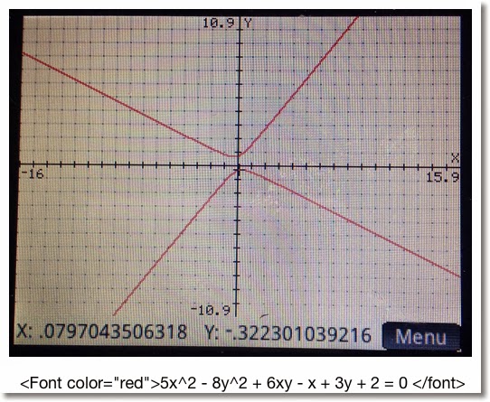
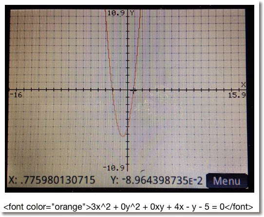
Below are some examples. Remember the form:

Ax^2 + By^2 + Cxy + Dx + Ey + F = 0

Projectile Motion for HP Prime

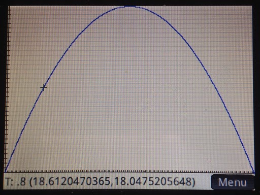
This program calculates range and height of a projectile, and plots its path. The program sets the mode into Degrees (HAngle=1) and the calculator to the Parametric app.

Equations:
x = V * cos θ * t
y = V * sin θ * t - .5 * g * t^2

Where
V = initial velocity
θ = initial degree of flight
g = Earth gravitation constant (9.80665 m/s^2, ≈32.17404 ft/s^2)

Air resistance is not factored, so we are dealing with ideal conditions. How much the projectile represents reality varies, where factors include the object being projected, the temperate and pressure of the air, and the weather.

EXPORT PROJ13()
BEGIN
LOCAL M, str;
// V, G, θ are global
// Degrees
HAngle:=1;

CHOOSE(M, "Units", "SI", "US");
IF M==1 THEN
str:="m";
G:=9.80665;
ELSE
str:="ft";
G:=32.17404;
END;

INPUT({V, θ}, "Data",
{"V:","θ:"},
{"Initial Velocity in "+str+"/s",
"Initial Angle in Degrees"});

X1:="V*COS(θ)*T";
Y1:="V*SIN(θ)*T-.5*G*T^2";

STARTAPP("Parametric");
CHECK(1);
// Adjust Window
Xmin:=0
// Range
Xmax:=V^2/G*SIN(2*θ);
Ymin:=0
// Height
Ymax:=(V^2*SIN(θ)^2)/(2*G);
MSGBOX("Range: "+Xmax+" "+str+", "
+", Height: "+Ymax+" "+str);
// Plot View
STARTVIEW(1,1);
END;

Below are screen shots from an example with V = 35.25 m/s and θ = 48.7°.

This concludes this session of the tutorials. Shortly I will have Part 6 up, which has to do routines.

I am catch-up mode, still. But then again I always feel like there is too much to do and too little time. LOL

See you soon!

Eddie


This blog is property of Edward Shore. 2013

HP Prime Programming Tutorial #4: CHOOSE and CASE, Tip about INPUT

Welcome to Part 4 of our programming series for the Prime. Today's session will cover CHOOSE and CASE.

---

First a tip from Han of the MoHPC Forum, which is found at http://www.hpmuseum.org/cgi-sys/cgiwrap/hpmuseum/forum.cgi#255084. Thank you Han for allowing me to share this.

Use the IF THEN ELSE structure with INPUT to execute a set of default instructions if the user presses cancel. INPUT returns a value of 0 if ESC or cancel is pressed, and 1 if a value is entered.

IF INPUT(...) THEN
commands if values are entered
ELSE
commands if Cancel is pressed
END;

Default values can be assigned to values as an optional fifth argument for INPUT.

INPUT(var, "Title", "Prompt", "Help", default value)

The type of variable maybe set to other than real numbers. Just remember to store such type before the INPUT command. For example, if you want var to be a string, store an empty string:

var:=" ";

Again, major thanks to Han.

---

CHOOSE and CASE

CHOOSE: Creates a pop up choose box, similar to what you see when you click on a soft menu. There are two syntaxes for CHOOSE:

Simple Syntax (up to 14 options):
CHOOSE(var, "title string", "item 1", "item 2", ... , "item n");

List syntax (infinite amount of items):
CHOOSE(var, "title string", {"item 1", "item 2"});

Choosing item 1 assigns the value of 1 to var, choosing item 2 assigns the value of 2 to var.

Access: Cmds, 6. I/O, 1. CHOOSE

---

CASE: Allows for different test cases for one variable. Also includes a default scenario (optional).

CASE
IF test 1 THEN do if true END;
IF test 2 THEN do if true END;
...
DEFAULT commands END;

Access: Cmds, 2. Branch, 3. CASE

Let's look at two programs to demonstrate both CHOOSE and CASE.

---

TERMVEL - Terminal Velocity of an Object

EXPORT TERMVEL()
BEGIN

LOCAL L0:={9.80665,32.174},
L1:={1.225,.0765},
L2:={.47,1.05,1.15,.04},C,K,M,A,T;

CHOOSE(C,"Units","SI","English");

CHOOSE(K,"Type of Object","Sphere","Cube",
"Cylinder","Tear-Shaped");

INPUT({M,A},"Object",
{"M=","A="},{"Mass","Surface Area"});

T:=√((2*M*L0(C))/(L1(C)*A*L2(K)));

MSGBOX("Terminal Velocity="+T);
RETURN T;
END;

---

Examples:

Sphere, SI Units, M = .05 kg, A = .0028 m^2
Terminal Velocity: T = 24.6640475387 m/s

Cube, US Units, M = 1.2 lb, A = .3403 ft^2
Terminal Velocity: T = 53.149821209 ft/s

---

AREAC - Area of Circles, Rings, and Sectors

EXPORT AREAC()
BEGIN
LOCAL C,R,S,θ,A;
CHOOSE(C,"Areas","1. Circle","2. Ring","3. Sector");

INPUT(R, "Input Radius", "R =");

CASE
IF C==1 THEN A:=π*R^2; END;

IF C==2 THEN
INPUT(S,"Small Radius","r=");
A:=π*(R^2-S^2);
END;

IF C==3
INPUT(θ, "Angle", "θ=");
\\ Assume you are in the correct angle mode
IF HAngle==1 THEN
\\ Test Angle Mode
θ:=θ*π/180;
END;
A:=θ*R^2/2;
END;

END;

MSGBOX("Area is "+A);
RETURN A;
END;

---

Examples

R = 2.5, r = 1.5, θ = π/4 radians or 45°

Circle: 19.6349540849
Ring: 12.5663706144
Sector: 2.45436926062

---

That is how, in general CHOOSE and CASE work. I thank you as always. It is so good to finally be rid of a cold and firing on all cylinders again.


Eddie

This blog is property of Edward Shore. 2013

HP Prime Programming Tutorial #3: WHILE, INPUT, KILL, REPEAT, GETKEY

This tutorial is going to cover a lot, each with some new programming commands in this series. I hope you are ready for the intensity. :)

---

WHILE, INPUT, KILL

HP Prime Program: TARGET. TARGET is a game where you provide a guess to get a desired number. If you miss, the calculator will tell you if number is higher and lower. At the end of the game, the calculator gives you how may picks you needed to get the target number.

WHILE: Repeat a number of commands while a specific condition is test.

WHILE condition is true DO
commands
END;

Access: Tmplt, 3. Loop, 5. WHILE

Caution: Watch your ENDs! Make sure an END is with each loop and the program itself. Press the soft key Check to check your work.

INPUT: Creates an input screen for variables. On the HP Prime, the input can asked for more than one input. TARGET demonstrates INPUT with one prompt.

One Variable:
INPUT(variable, "title", "label", "help text")
Multi-Variable:
INPUT(list of variables, "title", list of "labels", list of "help text")

Note: Pressing Cancel will store a 0 in variable. You may include code of what to do if the user presses Cancel, but it is not required.

Access: Cmds, 6. I/O, 5. INPUT

KILL: Terminates program execution. Nothing dies, I promise.

Access: Tmplt. 1. Block, 3. KILL

---

Program:
EXPORT TARGET()
BEGIN
LOCAL C:=0, N:=RANDINT(1,20), G:=-1;
WHILE G≠N DO
C:=C+1;
INPUT(G,"Guess?","GUESS:","1 - 20");

IF G==0 THEN
KILL;
END;

IF G < N THEN
MSGBOX("Higher");
END;

IF G > N THEN
MSGBOX("Lower");
END;

END;

MSGBOX("Correct! Score: "+C);

END;

---

Try it and of course, you can adjust the higher limit. Here is some thing for you to try with TARGET:

1. Add a limited amount of guesses.
2. Can you display the list of guesses?

---

REPEAT

ULAM Algorithm: take an integer n. If n is even, divide it by 2. If n is odd, multiply it by 3 and add 1. ULAM counts how many steps it takes to get n to 1.

REPEAT:

Access: Tmplt, 3. Loop, 6. REPEAT

Featured:
CONCAT(list1, list2): Melds list1 and list2 into one.

Access: Toolbox, Math, 6. List, 4. Concatenate

---

EXPORT ULAM(N)
BEGIN
LOCAL C:=1, L0:={N};

REPEAT

IF FP(N/2)==0 THEN
N:=N/2;
ELSE
N:=3*N+1;
END;

C:=C+1;
L0:=CONCAT(L0,{N});
UNTIL N==1;

MSGBOX("NO. OF STEPS="+C);
RETURN L0;
END;

---

Examples:

ULAM(5) returns:
Message Box: "NO. OF STEPS=6"
List: {5, 16, 8, 4, 2, 1}

ULAM(22) returns:
Message Box: "NO. OF STEPS=16"
List: {22, 11, 34, 17, 52, 26, 13, 40, 20, 10, 5, 16, 8, 4, 2, 1}

---

GETKEY

The next section will introduce a super-important command, GETKEY. We will be working with GETKEY over the entire series.

The Program KEYNO: The person presses key presses. Which each key press, the code returns to the terminal screen. The program terminates when the Enter key is pressed.

GETKEY: Returns the key code of last key pressed. The Prime's key map is below. (Picture is from the HP Prime User's Guide)

Access: Cmds, 6. I/O, 4. GETKEY

EXPORT KEYNO()
BEGIN
LOCAL K;
PRINT();
PRINT("Press any key to get its code.");
PRINT("Press Enter to exit.");

REPEAT
K:=GETKEY;
IF K ≥ 0 THEN
PRINT(K);
END;
UNTIL K==30;

END;

---

Example Key Codes:
33: 8 key
2: up
7: left
8: right
12: down
50: plus
45: minus

---

This concludes Part 3. Again, it can't be said enough, thanks for all the comments and compliments. And until next time,

Eddie


This blog is property of Edward Shore. 2013

HP Prime Tip: RPN and Created Programs

Major thanks to Miguel Toro from the MoHPC Forum for this tip:

There are two ways to call created programs in RPN mode of the HP Prime:

Vertically:
argument 1 [Enter]
argument 2 [Enter]
...
argument n [Enter]
program [Enter]

Horizontally:
argument 1 [space] argument 2 [space] ... argument n [space] program
[Enter]

Keep in mind this works with created user programs. To ensure that built-in commands work correctly, still include the number of arguments as needed.

Link to the forum: http://www.hpmuseum.org/cgi-sys/cgiwrap/hpmuseum/forum.cgi


Eddie


This blog is property of Edward Shore. 2013

Matrix Calculations: det(A - B * λ)=0

Let A and B be square matrices. B is a diagonal matrix. A diagonal matrix is a matrix with entries in it's diagonal positions, (1,1), (2,2), and so on, and 0 everywhere else. The identity matrix is a diagonal matrix. Another example is:

[ [2, 0, 0],[0, -2, 0],[0, 0, 5] ]

Let m, n, r, s, and t be numerical constants. Let a1, a2, and a3 be entries on the first row. Similar for b1, b2, b3, c1, c2, and c3.

det(A - B * ident(λ)) = 0

---

Comparison of 2 x 2 Matrices:
Note the constant term (λ^0), typed in green, the same.

B is a 2 x 2 identity matrix.

det( [ [a1, a2],[b1, b2] ] - λ * [ [1,0],[0,1] ] ) = 0
det( [ [a1, a2],[b1, b2] ] - [ [λ, 0],[0, λ] ]) = 0
λ^2 - (a1 + b2) * λ + a1*b2 - a2*b1 = 0

B is a diagonal matrix [ [m, 0],[0, n] ].

det( [ [a1, a2],[b1, b2] ] - λ * [ [m,0],[0,n] ] ) = 0
det( [ [a1, a2],[b1, b2] ] - [ [m*λ, 0],[0, n*λ] ]) = 0
m*n*λ^2 - (a1*n + b2*m)*λ + (a1*b2 - a2*b1) = 0

---

Comparison of 3 x 3 Matrices:
Note the constant term (λ^0), typed in green, the same.

B is a 3 x 3 identity matrix.

det( [ [a1,a2,a3],[b1,b2,b3],[c1,c2,c3] ] - λ * [ [1, 0, 0],[0, 1, 0],[0, 0, 1] ] ) = 0
det( [ [a1,a2,a3],[b1,b2,b3],[c1,c2,c3] ] - [ [λ, 0, 0],[0, λ, 0],[0, 0, λ] ] ) = 0

- λ^3
+ λ^2 * (a1 + b2 + c3)
+ λ * (-a1*b2 - a1*c3 - b2*c3 + a2*b1 + a3*c1 + b3*c2)
+ (a1*b2*c3 - a1*b3*c2 - a3*b2*c1 - a2*b1*c3 + a2*b3*c1 + a3*b1*c2) = 0

B is a general 3 x 3 diagonal matrix, [ [r, 0, 0],[0, s, 0],[0, 0, t] ].

det( [ [a1,a2,a3],[b1,b2,b3],[c1,c2,c3] ] - λ * [ [r, 0, 0],[0, s, 0],[0, 0, t] ] ) = 0
det( [ [a1,a2,a3],[b1,b2,b3],[c1,c2,c3] ] - [ [r*λ, 0, 0],[0, s*λ, 0],[0, 0, t*λ] ] ) = 0

- λ^3 * r*s*t
+ λ^2 * (s*t*a1 + r*t*b2 + r*s*c 3)
+ λ * (a1*b2*c3 - a1*b3*c2 - a3*b2*c1 - a2*b1*c3 + a2*b3*c1 + a3*b1*c2) = 0


Of course to get the eigenvalues (λ), solve the appropriate polynomial.

Hope this is helpful to those studying linear algebra or for those who are curious. This post was inspired from a program I was helping a fellow HP Prime programmer.

This post is dedicated to Michael de Estrada.


This blog is property of Edward Shore. 2013

HP Prime Programming Tutorial #2: MSGBOX, IF-THEN-ELSE, PRINT, FOR

Welcome to another programming tutorial for the HP Prime. In this session, we will cover MSGBOX, IF-THEN-ELSE, PRINT, and the FOR loop.

---

MSGBOX

MSGBOX: MSGOX takes a string a makes a pop-up message box. Program execution stops until you press a key to acknowledge the message.
Access: Cmds, 6. I/O, 8. MSGBOX

The program COMLOCK: Imagine that you are in charge of setting the combinations for the good, old-school combination locks. This program gives three digit combinations through the use of MSGBOX.

EXPORT COMLOCK()
BEGIN
LOCAL L0;
L0:=RANDINT(3,0,39);**
MSGBOX("SECRET: "+L0(1)+","+L0(2)+","+L0(3));
END;  
** Thanks to Thomas Lake for pointing out my typo.  Apologies for any inconvenience - Eddie (3/21/2014)

---

Other commands that are featured:

RANDINT(n, a, b) generates a list of n integers between a and b. You can leave n out if you desire a single random integer. Picks may be repeated.

The HP Prime's default list variables are designated L0 through L9.

---

Here is a sample output for COMLOCK:

IF-THEN-ELSE

IF-THEN-ELSE: Program structure:
IF condition THEN
do if the condition is true;
ELSE
do if the condition is false;
END;

Access: Tmplt, 2. Branch, 2. IF THEN ELSE

---

Tip: You can leave out the ELSE part if you only want to test to see if a condition is true. Access the simple IF-THEN structure by pressing Tmplt, 2. Branch, 1. IF THEN.

Access <, ≤, ==, etc. by pressing Shift, 6. Note that the double equals is needed to check equality.

---

PRINT

PRINT: The PRINT command prints a sting, result, or a combination of both onto the Prime's Terminal screen. If PRINT is used, the program will end on the terminal (text output) screen. Press a button to exit.

You can access the terminal screen at any time by pressing the ON button, holding it, and then pressing the Divide ( ÷ ) button.

Access: Cmds, 6. I/O, 9. PRINT

---

Tip: To clear the terminal screen, type PRINT(). This is a good way to clear the terminal screen and I usually use this at the beginning of any program if PRINT is going to be used later on.

---

The program QROOTS (yet one more quadratic solver, sorry for not being original guys and gals), demonstrates the use of IF-THEN-ELSE and PRINT.

Here I set the setting variable HComplex to 1, which allows for complex number results.

EXPORT QROOTS(A,B,C)
BEGIN
LOCAL D;
PRINT();
HComplex:=1;
D:=B^2-4*A*C;
IF D≥0 THEN
PRINT("Roots are real.");
ELSE
PRINT("Roots are complex.");
END;
PRINT((-B+√D)/(2*A));
PRINT((-B-√D)/(2*A));
END;

Examples:

QROOTS(1,5,8) returns:

Roots are complex.
-2.5+1.32287565553*i
-2.5-1.32287565553*i

QROOTS(2,-4,-8) returns:

Roots are real.
3.2360679775
-1.2360679775

---

FOR

This section will explore the basic FOR structure:

FOR variable FROM start TO end DO
commands;
END;

All the commands in the loop will be executed a set number of times. Each time a loop finishes, the variable increases by one. The loop terminates when variable=end.

Access: Tmplt, 3. LOOP, 1. FOR

---

The program SUMDIV takes any integer and adds up the sum of its divisors. For example, the divisors of 12 are 1, 12, 2, 3, 4, and 6. The sum is 28.

---

Featured Commands in SUMDIV:

idivis: idivis(integer) returns a sequence of all of the divisors if integer. Access: Toolbox, CAS, 5. Integer, 1. Divisors

Any CAS command used in programming will be preceded by "CAS." Not all CAS commands can be used in HP Prime programming at this time.

DIM: returns the dimensions of a sequence, string, or matrix. DIM must be used instead of SIZE to prevent a Bad Argument error.

For sequences or vectors, DIM returns the length in a list {length}.
For strings, DIM returns length as a number.
For matrices, DIM returns the list {number of rows, number of columns}.

Access: Cmds, 1. Strings, 9. DIM

---

The program:

EXPORT SUMDIV(N)
BEGIN
LOCAL S:=0,K,mdiv,ldiv;
mdiv:=CAS.idivis(N);
ldiv:=DIM(mdiv);
FOR K FROM 1 TO ldiv(1) DO
S:=S+mdiv(K);
END;
RETURN S;
END;  

** Thanks to Thomas Lake for pointing out that the variable "mat", which I had in this program was unnecessary.  - Eddie 3/21/2013

 

Examples:
SUMDIV(12) returns 28.
SUMDIV(24) returns 60.
SUMDIV(85) returns 108.

---

This concludes this part of the HP Prime Programming Tutorial.

HAPPY HALLOWEEN!

Eddie


This blog is property of Edward Shore. 2013

HP Prime Programming Tutorial #1: LOCAL, RETURN

Over the next month, maybe month and a half, I plan to post programming tutorials for the HP (Hewlett Packard) Prime.

If you have programmed with the HP 38G, 39g, or 39gii, this language will be similar to those. The programming language for the Prime is named the HP Prime Programming Language (HPPP).

Throughout this tutorial, I am going to use the latest version of the software.

How to start writing a program:

1. Press Shift + 1 (Program).
2. Press New. It is the second touch key.
3. Enter the name of the program. Pressing the ALPHA key twice will turn on UPPERCASE ΑLPHA-LOCK. Pressing ALPHA, Shift, ALPHA will turn on lowercase alpha-lock. To exit any lock, press the ALPHA key one more time. When happy with the name, press Enter.

---

Rules for Program Names:

1. Letters, numbers, and the underscore character (_) only.

2. The program name must start with a letter.

---

Structure of a HP Prime Program

A HPPP program is encased of an EXPORT - BEGIN - END structure. The layout is generally like this:

EXPORT program_name(arguments)
BEGIN
commands and comments go here
END;

Each line containing a command generally must end with a semicolon (;). A semicolon can by type by pressing ALPHA then the Plus key ( + ).

Comments can be typed. The are designated by two forward slashes. The slashes are typed by pressing the Divide key ( ÷ ). Anything in the line following the two slashes is ignored in running the program.

---

SQIN

Our first program is SQIN, because "Hello World" programs are so 2000s. SQIN takes a number, squares it, then calculates the reciprocal. In short we are defining a custom function:

SQIN(x) = 1/x^2

Commands:

RETURN: returns a result to the stack (home page). You can return numbers, lists, vectors, matrices, strings, or a combination of these times.
Access: Tmplt, 1. Block, 2. RETURN

All the program code in this tutorial series will be shown in Courier font.

EXPORT SQIN(X)
BEGIN
RETURN 1/X^2;
END;

---

Tip: You can check the syntax of the program just by pressing the Check soft key in the program editor. HP Prime will inform you if there is a syntax error and attempt to point you to the error. If there are no syntax errors, the Prime states "No errors in the program". I use the Check command all the time.

---

How to run the programs:

Home Mode - Textbook Entry,
Home Mode - Algebraic Entry,
CAS Mode:

Type the program name. Follow the name with parenthesis and enclose the required arguments.

Or use the Toolbox (top row of white keys, 2nd key from the left, it looks like a tool box), select the User touch key, select the program, and input the required arguments.

Home Mode - RPN Entry:

Enter each argument, separate each entry by pressing the Enter key. Type the name, and in the parenthesis state the number of arguments.

For example, if the program TEST has four arguments, the RPN stack would like this:

4: argument_1
3: argument_2
2: argument_3
1: argument_4
TEST(4) to run the program.

---

Examples to try with SQIN:

SQIN(5) returns .04
SQIN(36) returns .000771604938


The next program will demonstrate the concept of local variables.

---

MOPMT

LOCAL: Declares any variables to be local to the program. In other words, the variables are created, used, possibly displayed during program execution, and deleted at program termination.
Access: Tmplt, 4. Variable, 1. LOCAL

---

Tip: You can declare local variables and assign an initial value at the same time. For example: LOCAL K:=1; stores 1 in K and makes K a local variable.

---

MOPMT calculates the monthly payment of a loan. The arguments are: the loan amount (L), the interest rate (R), and the number of months (M).

EXPORT MOPMT(L,R,M)
BEGIN
LOCAL K:=R/1200;
K:=L*K/(1-(1+K)^-M);
RETURN "Payment ="+K;
END;

---

Tip: Use RETURN, TEXTOUT_P, and PRINT to return custom strings, which combine results, messages, and calculations. Parts are connected with a plus sign.

---

Examples:
MOPMT(4000, 9.5, 30) returns 150.317437565
MOPMT(370000, 3.5, 360) returns 1661.46534383

Try this and next time in the series I will highlight other things we can do with HPPP. Thanks!

Eddie

This blog is property of Edward Shore. 2013 

Program: Operations with Large Numbers (HP Prime)

Operations with Large Numbers

Large Factorial (Version 2) - HP Prime

EXPORT LFACT(N)
BEGIN
LOCAL K,S,A;
FOR K FROM 2 TO N DO
S:=S+LOG(K);
END;
RETURN { ALOG(FP(S)), IP(S) };
END;

This is an approximation! Results: {mantissa, exponent}. To be interpreted like this: mantissa * 10^exponent

Examples (compared with actual calculations with HP 50g):

55!
LFACT: 1.2696403353 * 10^73
Actual: 1.26964033537 * 10^73

65!
LFACT: 8.24765059247 * 10^90
Actual: 8.24765059208 * 10^90

75!
LFACT: 2.48091408072 * 10^109
Actual: 2.48091408114 * 10^109

125!
LFACT: 1.88267716466 * 10^209
Actual: 1.88267717689 * 10^209

245!
LFACT: 3.44638099725 * 10^480
Actual: 3.44638108855 * 10^480

525!
LFACT: 6.89080261728 * 10^1201
Actual: 6.89080262404 * 10^1201

875!
LFACT: 1.31677044437 * 10^2196
Actual: 1.31677038751 * 10^2196

Large Powers - HP Prime

EXPORT LPWR(X,Y)
BEGIN
LOCAL S;
S:=Y*LOG(X);
RETURN { ALOG(FP(S)), IP(S) };
END;

This is an approximation! Results: {mantissa, exponent}. To be interpreted like this: mantissa * 10^exponent

Examples (compared with actual calculations with HP 50g):
50^38
LPWR: 3.63797880819 * 10^64
Actual: 3.63797880709 * 10^64

102^68:
LPWR: 3.84425050422 * 10^136
Actual: 3.84425050254 * 10^136

58^124:
LPWR: 4.624568333 * 10^218
Actual: 4.62456834156 * 10^218

302^219:
LPWR: 1.32288017481 * 10^543
Actual: 1.32288017363 * 10^543




This blog is property of Edward Shore. 2013

Calculus Lesson: Area Between Curves

Area Between Two Curves

The general formula for finding the area between two curves is:

b
∫ T(x) - B(x) dx
a

I named the functions T(x) and B(x) specifically. T(x) represents the function "on top", while B(x) represents the function "on the bottom". In short, for x ∈ (a,b), T(x) ≥ B(x).

Here is an approach to use when finding areas between curves. A graphing calculator or mathematical software can be helpful in this procedure.

1. Draw the graphs. This is where a graphing calculator comes in handy.

2. Determine a and b, your limit points. Sometimes one or both of the limit points are found by finding the intersection of the two curves. Other problems will give you a third (or even fourth) condition. An example is x≥0, which makes one of our limit points x=0.

3. Determine which of the curves is T(x) and B(x). T(x) has greater numerical value than B(x) over the interval x ∈ (a, b).

4. Take the definite integral of T(x) - B(x). The result is your area.

b
∫ T(x) - B(x) dx = Area
a


About the examples and problem set: Please note that most examples in math textbooks, the numbers come out "nice and neat". Not so here, so I am using an HP Prime to demonstrate these examples and come up with answers. (any graphing calculator, HP, TI, Casio, all will do just fine!)

Example 1:

Find the area between:
y = -x^2 + 2
y = x^2 + 1

Here is a graph of the two curves:

Finding the limit points:

-x^2 + 2 = x^2 + 1
1 = 2*x^2
1/2 = x^2
Which implies x = -1/√2 and x = 1/√2

So our limit points are a = -1/√2 and b = 1/√2

From the graph we note that:
T(x) = -x^2 + 2
B(x) = x^2 + 1
and
T(x) - B(x) = -x^2 + 2 - (x^2 + 1) = -2*x^2 + 1

Taking the integral:

1/√2
∫ -2*x^2 + 1 dx ≈ 0.94281
-1/√2

So the area for Example 1 is about 0.94281.

Example 2:

Find the area between the two curves:
y = 2 cos x
y = x - 2
With the condition x≥0

First we graph the two curves:

The two graphs intersect when x>0. Since we are given the additional condition that x≥0, the lower limit for this problem is a=0.

To find the upper limit, we find intersection point:
2 cos x = x - 2
2 cos x - x + 2 = 0

Using a numeric solver on a calculator, we find that the intersection point is x ≈ 1.71419. (See, the numbers in these examples aren't always as "neat").

In the region x ∈ (0, 1.71419), we see that 2 cos x > x - 2. Hence:

T(x) = 2 cos x
B(x) = x - 2
and the area is approximately

1.71419
∫ 2 cos x - (x + 2) dx ≈ 3.93863
0

Problems to Try

Problem 1
Find the area between the curves of
y = x^2
y = 4

Problem 2

y = x^3
y = -3*x + 8
With the condition x≥0

Problem 3

y = 8*x^2 + 4*x - 6
y = x

Check your answers:
Areas are rounded to five decimal points:
1. 10.66667
2. 7.36017 (Hint: Upper Limit ≈ 1.51275)
3. 7.42101 (Hint: Use a calculator to find the limit points)


Any questions, please leave them in the comment box. Hope this is helpful and thanks!


Eddie


This blog is property of Edward Shore. 2013

HP 35S: Resistors in Series or Parallel (Portred from HP-33E)

Resistors in Series or Parallel
Source: HP-33E Student Engineering Applications, 1978
Original Calculator: HP-33S
Credit to Hewlett Packard Company
Ported to HP 35S by Eddie Shore, 10/10/2013

Instructions:
1. For each group of parallel or series resistors: press XEQ R.
2. At the Mode Prompt (INPUT M), enter 0 R/S for Parallel Resistors, 1 R/S for Series Resistors
3. Enter resistor values (assumed to be in Ohms) then press R/S.
4. To find the total, press XEQ R016.
5. Optional: Store the result in a variable for future use, as long is it not R.

Parallel Resistors: total resistance = 1/( 1/R1 + 1/R2 + ... )

Series Resistors: total resistance = R1 + R2 + ...


Program:
R001 LBL R
R002 0
R003 STO R
R004 SF 10 // press Left Shift, Flags, SF, decimal point, 0
R005 0=PAR 1=SER // equation
R006 PSE
R007 CF 10 // press Left Shift, Flags, CF, decimal point, 0
R008 INPUT M
R009 R/S
R010 RCL M
R011 x=0?
R012 XEQ R024
R013 R-down
R014 STO+ R
R015 GTO R009

R016 RCL R // total resistance
R017 RCL M
R018 x=0?
R019 XEQ R024
R020 CLx
R021 STO M
R022 R-down
R023 RTN

R024 R-down
R025 1/x
R026 ENTER
R027 RTN

Example 1:

Keystrokes:
1st Set:
XEQ R ENTER
0 R/S
120 R/S
240 R/S
120 R/S
XEQ R016
STO T

2nd Set:
XEQ R ENTER
0 R/S
320 R/S
400 R/S
XEQ R016
STO U
RCL+ T

Total Resistance: 225 7/9 ohms

Example 2:

XEQ R ENTER
0 R/S
30 R/S
60 R/S
XEQ R016 // Result: 20
STO T

XEQ R ENTER
1 R/S
RCL T R/S
80 R/S
XEQ R016 // Result: 100
STO T

XEQ R ENTER
0 R/S
RCL T R/S
40 R/S
XEQ R016

Total Resistance: 28 4/7 ohms

Interesting Base Conversions - Porting a 1975 HP 25 Program to the HP 35S

Sometimes simple is best.

Base N to Base 10
Source: HP 25 Applications, 1975, pg. 22
Credit to Hewlett Packard Company
10/8/2013

Instructions:
Store the base of the number to be converted in B.
Start with the left most integer, press XEQ B. For each successive integer, press R/S. This is the integer portion.
Start with the left most fractional part, press XEQ B016. For each successive fractional digit, press R/S.

Examples:
1777 base 8 → 1023
143.2044 base 5 → 48.4384
1.11011 base 2 → 1.84375
B3A.F base 16 → 3131.9375

Program:
B001 LBL B
B002 STO A
B003 RCL B
B004 ENTER
B005 ENTER
B006 ENTER
B007 RCL A
B008 R/S
B009 STO A
B010 CLx
B011 +
B012 x
B013 RCL A
B014 +
B015 GTO B008
B016 RCL B
B017 1/x
B018 STO C
B019 STO D
B020 x
B021 R/S
B022 RCL C
B023 RCL D
B024 x
B025 STO D
B026 x
B027 +
B028 GTO B021

Base 10 to Base N
Source: HP 25 Applications, 1975, pg. 24
Credit to Hewlett Packard Company
10/8/2013

Instructions:
1. Store the number to be converted in A
2. Store the desired base in B
3. Press R/S stop. The approximation will build and keep building indefinitely until stopped.

Examples:
67.32 → 4 03. 05 01 14 11 base 16 (≈43.51EA base 16)
π ≈ 11.001001 base 2

√2 ≈ 1.0110101 base 2

Program:
T001 LBL T
T002 RCL B
T003 10
T004 x≥y?
T005 GTO T007
T006 100
T007 STO C
T008 0
T009 STO D
T010 RCL A
T011 LN
T012 RCL B
T013 LN
T014 ÷
T015 x<0?
T016 GTO T019
T017 IP
T018 GTO T022
T019 IP
T020 1
T021 -
T022 STO E
T023 RCL C
T024 x<>y
T025 y^x
T026 RCL D
T027+
T028 STO D
T029 PSE
T030 RCL B
T031 RCL E
T032 y^x
T033 STO - A
T034 GTO T010


This blog is property of Edward Shore. 2013

Jeppesen E68 Wind Easy Computer

This past Sunday at the Pasadena City College Swap Meet, I found and bought a Jeppensen E6B Wind-Easy Computer. In reality, the E6B-2A is a slide rule specialized for aviation. The box may have not been in the best shape, how every he slide rule, its metal insert, instruction manual, and carrying pouch are all in great condition.

The E6B-2A has two sides: a calculator side and a wind side.

Though my schedule has not allowed me much time to work with the E6B-2A, from the manual each of the two sides of the slide rule allows for specific calculations.

Calculator Side:
* Computation of speed, distance, and time
* Distance conversions: kilometers, miles, and nautical miles, which each of the measuring guides marked on the outside scale.
* Altitude Calculations: Density and True Altitude
* True Air Speed
* Mach Speed
* Slide rule, where the outer and inner scales act as scales C and D, respectively.

Wind Side:
* Calculations involving the "wind triangle", made up of the wind vector, ground vector, and air vector.
* Using the wind charts to plot true speed and course.

I have never owned a slide rule like this before, very interesting and unique - and something to carve out some time to learn. Very cool item!

Eddie


This blog is property of Edward Shore. 2013

.

HP Prime Program: Sampling Without Replacement

SAMPLE - Generate a list of random integers from 1 to N using sample without replacement.

Author: Eddie Shore
Date: 10/1/2013

Syntax: SAMPLE(L, N)
L = length of desired list
N = high integer
If L > N, an error occurs.

Output: random sample

Program:
EXPORT SAMPLE(L,N)
BEGIN
// length, number
LOCAL I, K, T, num;

// error cond
IF L > N THEN
1/0;
END;

// main program
L1:=MAKELIST(0,X,1,L,1);
L1(1):=RANDINT(N-1)+1;
I:= 2;

REPEAT
num:=RANDINT(N-1)+1;
T:=1;

// test for uniqueness
FOR K FROM 1 TO I DO
IF num == L1(K) THEN
T:=T + 1;
END;
END;

IF T == 1 THEN
L1(I) := num;
I := I + 1;
END;

UNTIL I == L + 1;
RETURN L1;
END;

Examples:
SAMPLE(5,9) (length of 5, n = 9) can generate:
{5, 4, 8, 2, 6}
{9, 7, 8, 1, 2}
{4, 3, 6, 5, 2}


This blog is property of Edward Shore. 2013