Showing posts with label electricity. Show all posts

Saturday, February 1, 2025

TI-84 Plus CE and DM42: RLC Circuits

TI-84 Plus CE and DM42: RLC Circuits


The program RLC calculates:


(1) The total impedance across the entire circuit

(2) The phase angle, sometimes known as a power factor angle

(3) The total supply current


An RLC circuit is a circuit that connects one power supply to a resistor, an inductor, and a capacitor. The resistor, inductor, and capacitor can be connected in one of two ways: series or parallel. To calculate the total impedance (Z) and phase angle (θ), the rectangular to polar conversion function can be utilized.


In a general rectangular to polar conversion, (x, y) to (r, θ):

r = √(x^2 + y^2)

θ = arctan(y / x)


Formulas


Angular Frequency: ω = 2 * π * F


F = frequency in Hz

V = supply voltage (volts)

R = resistor in Ω (ohms)

L = inductor in H (henrys)

C = capacitance (farads)

I = overall current (amps)

Series RLC Circuit - Formulas


Z = √(R^2 + (ω*L – 1 / (ω*C))^2)

θ = arctan ( (ω*L – 1 / (ω*C)) / R)

I = V / Z

Series RLC Circuit – Set up for Rectangular to Polar Conversion


x = ω*L – 1 / (ω*C)

y = R


Z = r

Parallel RLC Circuit - Formulas


1 / Z = √( (1/R)^2 + (1/(ω*L) – ω*C)^2)

θ = arctan ( (1/(ω*L) – ω*C) / (1/R))

I = V / Z

Parallel RLC Circuit – Set up for Rectangular to Polar Conversion


x = 1/(ω*L) – ω*C

y = 1/R


Z = 1/r


TI-84 Plus Program: RLC


ClrHome

Disp “RLC CIRCUIT”

Input “SUPPLY VOLTAGE? “, V

Input “FREQUENCY (HZ)? “, F

Input “RESISTANCE (OHMS)? “, R

Input “INDUCTOR (HENRYS)? “, L

Input “CAPACITOR (FARADS)? “, C

a+bi

Degree

2*π*F → W

Menu(“TYPE”, “SERIES”, 1, “PARALLEL”, 2)


Lbl 1

R+i*(W*L-1/(W*C)) → Z

abs(Z) → N

Goto 3


Lbl 2

(1/R)+i*(1/(W*L)-W*C) → Z

abs(Z)⁻¹ → N


Lbl 3

angle(Z) → θ

V/N → I


ClrHome

Disp “IMPEDANCE:”, N

Disp “PHASE ANGLE:”, θ

Disp “SUPPLY CURRENT:”, I


DM42, HP 42S Program: RLC


00 { 216-Byte Prgm }
01▸LBL "RLC"
02 "SUPPLY VOLTAGE?"
03 PROMPT
04 STO 01
05 "FREQUENCY?"
06 PROMPT
07 STO 02
08 "RESISTANCE?"
09 PROMPT
10 STO 03
11 "INDUCTOR?"
12 PROMPT
13 STO 04
14 "CAPACITOR?"
15 PROMPT
16 STO 05
17 DEG
18 2
19 STO 06
20 PI
21 STO× 06
22 RCL 02
23 STO× 06
24 "TYPE?"
25 AVIEW
26 PSE
27 "SERIES"
28 KEY 1 GTO 01
29 "PARA."
30 KEY 2 XEQ 02
31 MENU
32▸LBL 00
33 STOP
34 GTO 00
35▸LBL 01
36 CLMENU
37 EXITALL
38 RCL 06
39 RCL× 04
40 RCL 06
41 RCL× 05
42 1/X
43 -
44 RCL 03
45 →POL
46 STO 07
47 GTO 03
48▸LBL 02
49 CLMENU
50 EXITALL
51 RCL 06
52 RCL× 04
53 1/X
54 RCL 06
55 RCL× 05
56 -
57 RCL 03
58 1/X
59 →POL
60 1/X
61 STO 07
62▸LBL 03
63 "PHASE:"
64 AVIEW
65 PSE
66 VIEW ST Y
67 STOP
68 "IMPEADANCE:"
69 AVIEW
70 PSE
71 VIEW ST X
72 STOP
73 RCL 01
74 RCL÷ 07
75 "SUPPLY CURRENT:"
76 AVIEW
77 PSE
78 VIEW ST X
79 .END.


Examples


Examples are rounded to five digits.


Series Circuit


Inputs:


SUPPLY VOLTAGE: 300 V

FREQUENCY: 70 Hz

RESISTANCE: 80 Ω

INDUCTOR: 0.09 H

CAPACITOR: 150 μF (150E-6)


Results:


IMPEDANCE (Z) ≈ 83.64599 Ω

PHASE ANGLE (θ) ≈ 16.97904°

CURRENT (I) ≈ 3.58654 A


Parallel Circuit


Inputs:


SUPPLY VOLTAGE: 240 V

FREQUENCY: 90 Hz

RESISTANCE: 60 Ω

INDUCTOR: 20 mH (20E-3)

CAPACITOR: 140 μF (140E-6)


Results:


IMPEDANCE (Z) ≈ 52.46010 Ω

PHASE ANGLE (θ) ≈ 29.05363°

CURRENT (I) ≈ 4.57491 A


Sources


“Impedance and Complex Impedance” https://www.electronics-tutorials.ws/accircuits/impedance.html


“Parallel RLC Circuit Analysis” https://www.electronics-tutorials.ws/accircuits/parallel-circuit.html


“Series RLC Circuit Analysis” https://www.electronics-tutorials.ws/accircuits/series-circuit.html


Electronics Tutorials. AspenCore, Inc. 2024. Retrieved October 7, 2024 and October 17, 2024.


Eddie


All original content copyright, © 2011-2025. Edward Shore. Unauthorized use and/or unauthorized distribution for commercial purposes without express and written permission from the author is strictly prohibited. This blog entry may be distributed for noncommercial purposes, provided that full credit is given to the author.

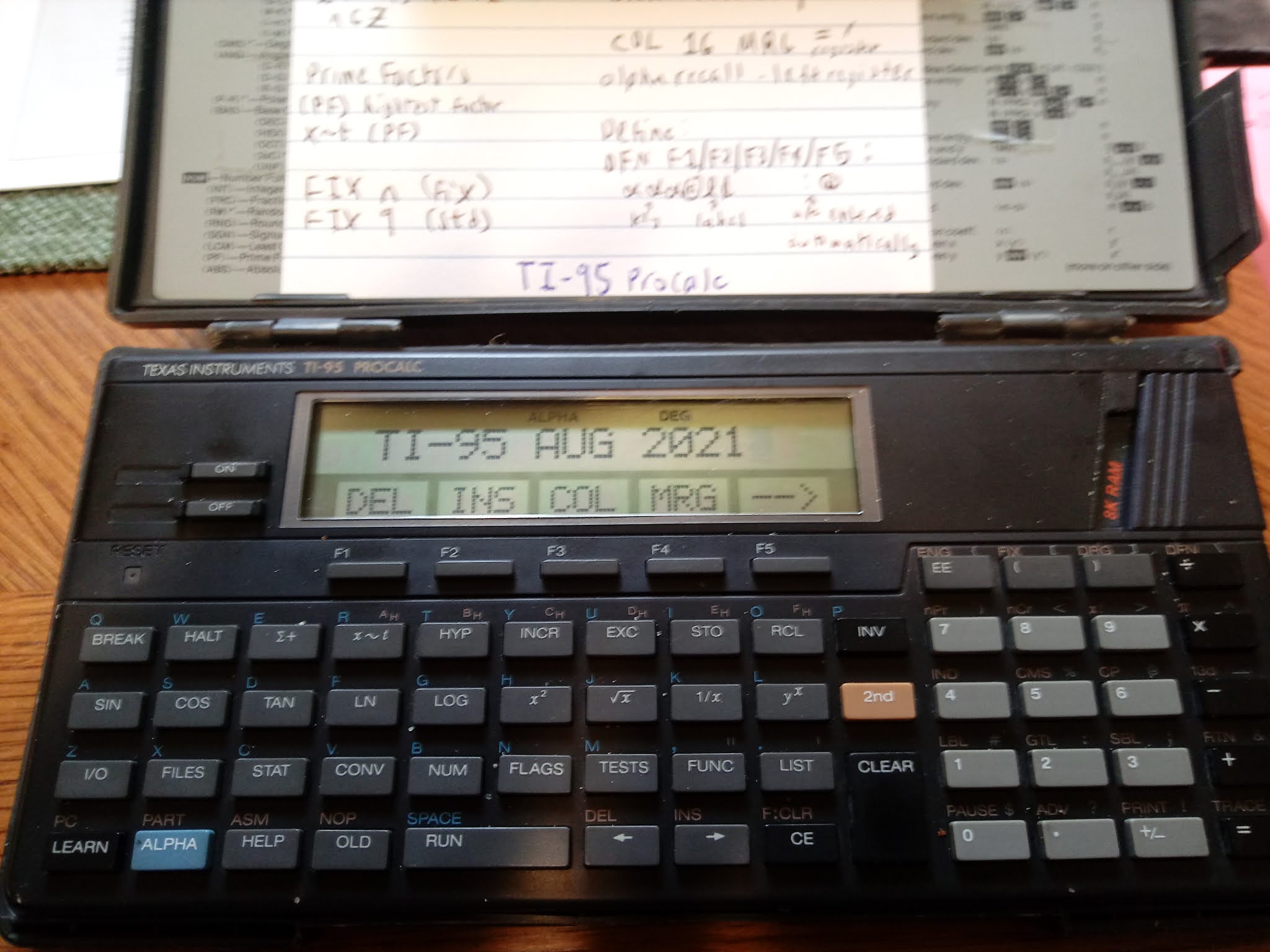
Saturday, August 14, 2021

TI-95 ProCalc: Solving Equations With 2 Known Values, Solve for the Third Variable


TI-95 ProCalc: Solving Equations With 2 Known Values, Solve for the Third Variable 


Introduction

The two programs presented on today's blog will show an approach to program a solver where:

*  Values for two variables are known
*  The third variable is solved for automatically

We will make use of TI-95 ProCalc's user flags 01, 02, and 03 to determine which variable has entries and which variable is to be solved for.   I stored 2 into a variable (in this case, C) to count down the number of values are entered.  These programs assume that the user will always enter values for two different variables without the need to review or edit values entered.

Keys:
F1:  first variable - controlled by user flag 01
F2:  second variable - controlled by user flag 02
F3:  third variable - controlled by user flag 03

TI-95 ProCalc's flag operations:
RF:  reset flag, clear flag
SF:  set flag
TF:  tests whether a flag is set
INV TF: tests whether a flag is reset

All the variables and their values, entered or solved for, are shown at the end.

Ohm's Law

R = V / I
R = resistance in Ohms (Ω)
V = voltage in Volts (V)
I = current in Amps (A)

The program reminds the user of what units are expected in the beginning.

CHAR 244 adds Ω to the alpha string.

The alpha string '   TO ENTER' has three spaces at the beginning of the string to allow room for C.   C is merged at space 2.  

Housekeeping Items: 

RF 01 RF 02 RF 03:  Resets the flags 01, 02, and 03 at the end of the program. 

DFN CLR:  Clears the defined keys F1 - F5. 

TI-95 ProCalc File OHM
Size:  224 bytes

0 STO I STO R STO V 2 STO C

RF 01 RF 02 RF 03 CLR

'OHM'S LAW' PAU CLR

'UNITS: ' CHR 244 ',A,V' PAU

LBL A0   

CLR '   TO ENTER'  COL 02 MRG C

DEF F1: R @A1  

DEF F2: I @A2

DEF F3: V @A3

HLT 

LBL A1 STO R SF 01 DSZ C GTL A0 GTL B0

LBL A2 STO I ST 02 DSZ C GTL A0 GTL B0

LBL A3 STO V SF 03 DSZ C GTL A0 GTL B0

LBL B0 

INV TF 01 SBL B1

INV TV 02 SBL B2

INV TF 03 SBL B3

CLR 'R=' COL 16 MRG R BRK

CLR 'I=' COL 16 MRG I BRK

CLR 'V=' COL 16 MRG V  RF 01 RF 02 RF 03 DFN CLR HLT

LBL B1 RCL V / RCL I = STO R RTN

LBL B2 RCL V / RCL R = STO I RTN

LBL B3 RCL I * RCL R = STO V RTN


Examples

I = 10 A, R = 1500 Ω;  Result:  V = 15,000 V

R = 200 Ω, V = 240 V; Result:  I = 1.2 A

I = 15 A, V = 110 V; Result: = 7.333333333 Ω


Right Triangle

This programs solves any of the following variables, from knowing the other two vales: 

X:  run
Y:  rise
R:  hypotenuse

In addition, the angle (Θ) is calculated where Y is considered the opposite side and X the adjacent side.

CHECK ANG MODE:  a prompt to check angle mode, just in case you are not in the desired angle mode.   The program runs in any angle mode.

CHR 242: adds Θ to the alpha string

TI-95 ProCalc File TRI
Size:  248 bytes

0 STO X STO Y STO R STO A 2 STO C

RF 01 RF 02 RF 03 CLR

'CHECK ANG MODE' BRK 

LBL A0   

CLR '   TO ENTER'  COL 02 MRG C

DEF F1:ADJ@A1  

DEF F2:ADJ@A2

DEF F3:HYP@A3

HLT 

LBL A1 STO X SF 01 DSZ C GTL A0 GTL B0

LBL A2 STO Y ST 02 DSZ C GTL A0 GTL B0

LBL A3 STO R SF 03 DSZ C GTL A0 GTL B0

LBL B0 

INV TF 01 SBL B1

INV TV 02 SBL B2

INV TF 03 SBL B3

( RCL Y / RCL X ) INV TAN = STO A

CLR 'X=' COL 16 MRG X BRK

CLR 'Y=' COL 16 MRG Y BRK

CLR 'R=' COL 16 MRG R BRK

CLR CHR 242 '=' COL 16 MRG 

A RF 01 RF 02 RF 03 DFN CLR HLT

LBL B1 ( RCL R x^2 - RCL Y x^2 ) SQR = STO X RTN

LBL B2 ( RCL R x^2 - RCL X x^2 ) SQR  = STO Y RTN

LBL B3 ( RCL X x^2 + RCL Y x^2 ) SQR = STO R RTN

Examples

All examples are in degrees mode.

X = 3, Y = 4
Results:  R = 5, Θ = 53.13010235°

X = 11.8, R = 19.9
Results:  Y = 16.02404443, Θ = 53.63231539°

Y = 27, R = 54.4
Results:  X = 47.22668737, Θ = 29.75706329°

Commas added to the results for readability.  

Eddie

All original content copyright, © 2011-2021.  Edward Shore.   Unauthorized use and/or unauthorized distribution for commercial purposes without express and written permission from the author is strictly prohibited.  This blog entry may be distributed for noncommercial purposes, provided that full credit is given to the author. 


Saturday, April 10, 2021

Fun with the HP 20S (April 10, 2021 Edition)

 Fun with the HP 20S (April 10, 2021 Edition)


In all the programs presented on the blog, all inputs are stored in the appropriate registers before the program is run.  


The Power of a Windmill


This program calculates the power generated by a windmill, given the diameter and velocity of the windmill’s fans.   SI units (meters, kilograms, seconds) are used.   The general equations used are:


Area of the swept by the windmill’s fans (in m^2):

A = ( π * diameter^2 ) / 4 


Power generated (in W (Watts), J/s, m^2 kg/s^3):

P = ½ * area * density * velocity^3 


Density of air = 1.225 kg/m^3


Input:

R1 = diameter of the fans, m 

R2 = velocity of the fans, m/s 


Output:

R3 = area that the fans cover, m^2;  press [ R/S ]

R4 = power of the fan, W


Program:

01 LBL A         61,41, A

02 RCL 1         22, 1

03 x² 51, 11

04 × 55

05 π 61, 22

06 ÷ 45

07 4 4

08 = 74

09 STO 3         21, 3

10 R/S 26

11 × 55

12 RCL 2         22, 2

13 y^x 14

14 3 3

15 × 55

16 . 73

17 6 6

18 1 1

19 2 2

20 5 5

21 = 74

22 STO 4         21, 4

23 RTN 61, 26


Example:

Inputs:  

diameter = R1 = 6.65 m

velocity = R2 = 10 m/s

Results:

R3 = area = 34.7322702808 m^2

R4 = power = 21,273.515547 W


Source:

Sharp Electronics Corporation.  Conquering The Sciences: Applications for the SHARP Scientific Calculators EL-506P, EL-510S, EL-515S  Japan. 1984


Depth of a Well


This program calculates the depth of a well, which is determined by the time between a person drops a rock and the person hears the rock hit the bottom of the well.  The program uses SI units (meters, kilograms, seconds) with the following constants:


Earth’s Gravitational Acceleration:  g = 9.80665 m/s^2

g/2 = 4.903325 m/s^2

Speed of Sound, in dry air, 20°C temperature: s = 343.21 m/s


Equations:

X = (-B + √(B^2 + 4*A*B)) / 2

Y = g/2 * a^2


where:

B = s / (g/2) (see the above constants)

A = amount of time, in seconds, between the person drops the rock and hears the rock hit the bottom (input)

X = amount of time, in seconds, that it actually takes the rock from the time it was dropped until the rock hits the bottom of the well (output)

Y = depth of the well, in meters (output)


Input:

R1 = time until you hear the rock hit the bottom of the well (sec) 

Output:

R2 = time until the rock actually hits the bottom of the well (sec), [ R/S ]

R3 = depth of the well (m)


Program:

01 LBL B         61, 41, B

02 3 3

03 4 4

04 3 3

05 . 73

06 2 2

07 1 1

08 ÷ 45

09 4 4

10 . 73

11 9 9

12 0 0

13 3 3

14 3 3

15 2 2

16 5 5

17 STO 0         21, 0

18 = 74

19 STO 4         21, 4

20 +/- 32

21 + 75

22 ( 33

23 RCL 4         22, 4

24 x² 51, 11

25 + 75

26 4 4

27 × 55

28 RCL 4         22, 4

29 × 55

30 RCL 1         22, 1

31 ) 34

32 √ 11

33 = 74

34 ÷ 45

35 2 2

36 = 74

37 STO 2         21, 2

38 R/S 26

39 x² 51, 11

40 × 55

41 RCL 0         22, 0

42 = 74

43 STO 3         21, 3

44 RTN 61, 26


Example:

Input:  

time until you hear the rock hit the ground = R1 = 3 sec

Results:

R2 = time the rock travels to the bottom of the well = 2.8813865 sec

R3 = depth of the well = 40.70930098622 m


Source:

Saul, Ken.  The Physics Collection:  Ten HP-41C Programs for First-Year Physics Class   Corvallis, OR.  1986


Thevenin’s Theorem


This program calculated the equivalent resistance and voltage of a linear network of two resistors and a capacitor.  


Formulas:

R_TH = (R1 * R2) / (R1 + R2)

V_TH = V * R2 / (R1 + R2)


Inputs:

R1 = resistor 1 ( Ω )

R2 = resistor 2 ( Ω )

R3 = capacitor ( V )

Output:

R4 = equivalent resistor, R_TH, [ R/S ]

R5 = equivalent capacitor, V_TH


Program:

01 LBL C         61, 41, C

02 RCL 1         22, 1

03 × 55

04 RCL 2         22, 2

05 ÷ 45

06 ( 33

07 RCL 1         22, 1

08 + 75

09 RCL 2         22, 2

10 ) 34

11 = 74

12 STO 4         21, 4

13 R/S 26

14 RCL 3         22, 3

15 × 55

16 RCL 2     22, 2

17 ÷ 45

18 ( 33

19 RCL 1     22, 1

20 + 75

21 RCL 2         22, 2

22 ) 34

23 = 74

24 STO 5     21, 5

25 RTN 61, 26


Example:

Input:

R1 = 8 Ω

R2 = 9 Ω

R3 = 11 V

Results: 

R4 = 4.23529411765 Ω

R5 = 5.82352941176 V


Source:

Gussow, Milton and William T. Smith  Schaum’s Easy Outlines: Basic Electricity  New York. 2012  ISBN 978-0-07-178068-1


Norton’s Theorem


This program calculates an equivalent resistance and current when any network connected to a positive and a negative terminal.


Formulas:

R_N = (R1 * R2) / (R1 + R2)

I_N = V / R1


Inputs:

R1 = resistor 1 ( Ω )

R2 = resistor 2 ( Ω )

R3 = capacitor ( V )

Output:

R4 = equivalent resistor, R_N, [ R/S ]

R5 = equivalent current, I_N

Program:

01 LBL D         61, 41, D

02 RCL 1         22, 1

03 × 55

04 RCL 2         22, 2

05 ÷ 45

06 ( 33

07 RCL 1         22, 1

08 + 75

09 RCL 2         22, 2

10 ) 34

11 = 74

12 STO 4         21, 4

13 R/S 26

14 RCL 3         22, 3

15 ÷ 45

16 RCL 1         22, 1

17 = 74

18 STO 5         21, 5

19 RTN 61, 26


Example:

Input:

R1 = 8 Ω

R2 = 9 Ω

R3 = 11 V

Results: 

R4 = 4.23529411765 Ω

R5 = 1.375 A


Source:

Gussow, Milton and William T. Smith  Schaum’s Easy Outlines: Basic Electricity  New York. 2012  ISBN 978-0-07-178068-1


Eddie 


All original content copyright, © 2011-2021.  Edward Shore.   Unauthorized use and/or unauthorized distribution for commercial purposes without express and written permission from the author is strictly prohibited.  This blog entry may be distributed for noncommercial purposes, provided that full credit is given to the author.


HP 67 Collection: October 2026

HP 67 Collection: Oct ober 2026 All examples are done in FIX 4. (DSP 4) Earth's Gravity at a Specific Latitude The true ea...