Sunday, November 15, 2015

The Series ( ((((0 + 1)^-1 + 1)^-1 + 1)^-1 + 1)^-1 + 1)^-1 + … + 1)^-1 and Fibonacci Numbers

The Series ( ((((0 + 1)^-1 + 1)^-1 + 1)^-1 + 1)^-1 + 1)^-1 + … + 1)^-1 and Fibonacci Numbers


Add One Then Reciprocate

Define the series t as:

t = ( ((((0 + 1)^-1 + 1)^-1 + 1)^-1 + 1)^-1 + 1)^-1 + … + 1)^-1    (an infinite amount of terms)

This is a sum that can’t be easily stated in summation statement (Σ f(x)). 

On the HP Prime, I programmed this as:

EXPORT TEST1112(n)
BEGIN
LOCAL k, t:=0;
FOR k FROM 1 TO n DO
t:=(t+1)^-1;
END;
RETURN t;
END;

The result seems to converge at 0.6180339785 when n ≥ 27.  Note that 0.6180339785 = ϕ – 1, where ϕ is the Golden Ratio ( ϕ = (√5 + 1)/2)


Fibonacci Gets Involved

Note that:

k =
t =
1
1
2
(1 + 1)^-1 = 1/2
3
(1 + 1/2)^-1 = (3/2)^-1 = 2/3
4
(1 + 2/3)^-1 = (5/3)^-1 = 3/5
5
(1 + 3/5)^-1 = (8/5)^-1 = 5/8
6
(1 + 5/8)^-1 = (13/8)^-1 = 8/13
7
(1 + 8/13)^-1 = (21/13)^-1 = 13/21

We get a sequence of terms {1, 1/2, 2/3, 3/5, 5/8, 8/13, 13/21, 21/34, 34/55, 55/89, 89/144, …} where each term takes the fraction a/b, a is the kth Fibonacci number and b is the (k+1)th Fibonacci number.  Can we show that this sequence of partial sums is convergent?

Each partial sums of the series takes the form F_k / F_k+1 where F is the Fibonacci number.

The closed formula for the Fibonacci number is:

F_k = ( ϕ^k – α^k )/√5 , where ϕ  = (1 + √5)/2 and α = (1 - √5)/2.

Then:

F_k / F_k+1
=( ϕ^k – α^k )/√5 * √5/( ϕ^k+1 – α^k+1)
=( ϕ^k – α^k) / ( ϕ^k+1 – α^k+1 )
= ( ϕ^k / ϕ^k+1) * ( (1 – (α/ϕ)^k) / (1 – (α/ϕ)^k+1) )
= 1/ϕ * ( (1 – (α/ϕ)^k) / (1 – (α/ϕ)^k+1) )

Note that α/ϕ = (1 - √5)/(1 + √5 ) ≈ -0.38197 < 1

As k → ∞,  α/ϕ → 0. 

Hence,

lim k → ∞ (F_k / F_k+1)
= lim k → ∞ (1/ϕ * ( (1 – (α/ϕ)^k) / (1 – (α/ϕ)^k+1) ) )
= 1/ϕ

Simplifying:

1/ϕ
= 2/(1 + √5)
= 2*(1 - √5) / ((1 + √5)*(1 - √5))
= 2*(1 - √5)/-4
= (√5 – 1)/2
= √5/2 – 1/2

Adding and subtracting 1/2:

√5/2 – 1/2 + (1/2 – 1/2)
= (√5 + 1)/2 – 1
= ϕ – 1

Since the sequence of partial sums converge to ϕ – 1, the series

t = ( ((((0 + 1)^-1 + 1)^-1 + 1)^-1 + 1)^-1 + 1)^-1 + … + 1)^-1   

converges to ϕ – 1.


This blog is property of Edward Shore.  2015.


Monday, November 9, 2015

HP Prime Geometry App Tutorial Part 8: Rotating Triangles

HP Prime Geometry App Tutorial Part 8:  Rotating Triangles

Today’s lesson will show how to rotate a triangle given an angle.  The angle is in a counter-clockwise direction. 

For the purpose of this lesson, we will set the HP Prime in Degrees mode.

Draw the Triangle

1.  Set the calculator to Degrees mode.  Draw a triangle with vertices (4,4), (4, -4), and (8, 0). 

Rotate the Triangle

2.  Press (Cmds), 7 for Transformation, 3 for Rotation. 
3.  Select the reference point.  In our example, let’s make this point (0,0) and press [ Enter ].
4.  You are asked for an angle.  Enter 90 for 90°.  Press [ Enter ].


More Rotation

5.  Repeat steps 2 through 4, for angles of 180 and 270.


Thank you.  Until next time, have a great day!

Eddie

This blog is property of Edward Shore.  2015.


HP Prime Geometry App Tutorial Part 7: Conic Sections and Equations

HP Prime Geometry App Tutorial Part 7: Conic Sections and Equations

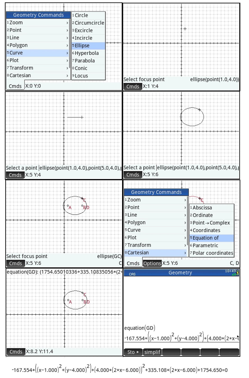
In today’s lesson we will work conic sections and showing the equations for each of the conic sections.

Drawing an Ellipse and Display its Equation

Command:  ellipse(focus point 1, focus point 2, point on the ellipse)

Draw an ellipse with foci (1,4) and (5,4) and the point on the ellipse on (5,6).

1.  Press (Cmds), 5 for Curve, 5 for Ellipse. 
2.  Go to the point (1,4) and press [ Enter ].
3.  Go to the point (5,4) and press [ Enter ].
4.  Go to the point (5,6) and press [ Enter ].

The next step is to display its equation. 

5.  Press (Cmds), 8 for Cartesian, 5 for Equation of.
6.  Select the ellipse and press [ Enter ].  In this example the equation is named GD.
7.  To see the whole equation, press [ CAS ] and execute the equation(GD) command.
8.  Press the up button to highlight the equation and press (Show).  Scroll to see the entire equation.


Drawing a Hyperbola and Display its Equation

Command:  hyperbola(focus point 1, focus point 2, point on the hyperbola)

Drawn a hyperbola with foci (-2, -2) and (-4, 2) with point (-9, 2).

1.  Press (Cmds), 5 for Curve, 6 for Hyperbola. 
2.  Go to the point (-2,-2) and press [ Enter ].
3.  Go to the point (-4,-2) and press [ Enter ].
4.  Go to the point (-9,2) and press [ Enter ].

The next step is to display its equation. 

5.  Press (Cmds), 8 for Cartesian, 5 for Equation of.
6.  Select the ellipse and press [ Enter ].  In this example the equation is named GD.
7.  To see the whole equation, press [ CAS ] and execute the equation(GD) command.
8.  Press the up button to highlight the equation and press (Show).  Scroll to see the entire equation.


Drawing a Parabola and Display its Equation

Command:  parabola(focus point, directrix line)

Draw a parabola with focus point (0,-5) and (0,3) is on the directrix line.

1.  Press (Cmds), 5 for Curve, 7 for Parabola. 
2.  Go to the point (0,-5) and press [ Enter ].
3.  Go to the point (0,3) and press [ Enter ].

The next step is to display its equation. 

4.  Press (Cmds), 8 for Cartesian, 5 for Equation of.
5.  Select the ellipse and press [ Enter ].  In this example the equation is named GC.
6.  To see the whole equation, press [ CAS ] and execute the equation(GC) command.
7.  Press the up button to highlight the equation and press (Show).  Scroll to see the entire equation.


On the next part, we will work with rotating geometric objects.   Thank you and see you next time,

Eddie


This blog is property of Edward Shore – 2015.  

HP Prime Geometry App Tutorial Part 6: Polygons

HP Prime Geometry App Tutorial Part 6:  Polygons

Drawing a Regular Polygon

1.  Clear the Plot screen.  Press (Cmds), 4 for Polygon, 9 for Regular Polygon. 
2.  Select one corner and press [ Enter ].
3.  Select another corner point and press [ Enter ].
4.  Enter the number of sides of the regular polygon.


Drawing a General Polygon

1.  Press (Cmds), 4 for Polygon, 8 for Polygon.
2.  Start with a corner point and press [ Enter ].  Keep going choosing corner points and pressing [ Enter ]. 
3.  When you finished plotting the final corner point, press [ Enter ] one last time.  This connects the last corner point with the first corner point.   Hence, it is like go to the final point and press [ Enter ] twice.


Finding Areas of the Polygon

To recall, press (Cmds), 9 for Measure, 5 for Area.  Select a polygon (when selected they turned red) and press [ Enter ].


Next time, we will work with conic sections.   Have a great day,

Eddie

This blog is property of Edward Shore – 2015.


Sunday, November 8, 2015

Speed Test: Casio fx-991EX Classwiz vs Canon F-792SGA

Speed Test:  Casio fx-991EX Classwiz vs Canon F-792SGA

https://www.youtube.com/watch?v=39tcSQBakMo


Eddie


This blog is property of Edward Shore.  2015

HP Prime Geometry App Tutorial Part 5: Plotting Functions and Differential Equations

HP Prime Geometry App Tutorial Part 5:  Plotting Functions and Differential Equations

The Geometry App can plot functions, parametric functions, polar functions, sequences, implicit statements, slope-field and ordinary differential equations, lists, and designate sliders.   

In this lesson, we will demonstrate three types of plots.   For the purpose of the tutorial, clear the Plot screen before each example.

Plotting Functions ( y = f(x))

Plot y = e^x + 1.

1.  Press (Cmds), 6 for Plot, 1 for Function. 
2.  Type e^(x) + 1.  Press (OK).

Use the lowercase x.  The format is plotfunc( y(x) ).


Plot an Ordinary Differential Equation  (y’ = dy/dx = f(x,y))

Plot y’ = y*e^x +1 with the initial condition (1,1).

1.  Press (Cmds), 6 for Plot, 7 for ODE.
2.  Type y*e^(x)+1.   Note that x and y are in lowercase.
3.  Press [ , ] and type [x,y].   Here you designate which variable is independent and which is dependent.
4.  Press [ , ] and type  [1,1].  This is your initial conditions.  Press (OK), 

The entire format is plotode( f(x,y),  [x, y], [x0, y0])


Plot a Parametric Equation  ( x(t) + i*y(t) where i = √-1)

Plot x = 3t + 1, y = 2t – 1.   The format to be used is (3t + 1) + i*(2t -1).

‘1. Press (Cmds), 6 for Plot, 2 for Parametric.
‘2. Type (3t + 1) + i*(2t -1) and press ( OK ).

The entire format is plotparam( x(t) + i*y(t), var = tbeg..tend, tstep=step).  The t is in lowercase and the last two arguments, interval and step, are optional.


In Part 6 we’ll be plotting and working with polygons.   Thanks and take care,

Eddie


This blog is property of Edward Shore.  2015. 


HP Prime Geometry App Tutorial Part 4: Tangent Lines and Changing the Color of Objects

HP Prime Geometry App Tutorial Part 4:  Tangent Lines and Changing the Color of Objects

Plotting Lines Tangent to a Circle’s Point

1.  Start with a clear plot screen.   Draw a circle:  the location of its center and size is up to you.
2.  Press (Cmds), 3 for Line, 6 for Tangent. 
3.  Select a point on the circle and press [ Enter ].  The point is designated as object GD. 
4.  If you wish, display the coordinates of GD.  See Part 3 as a refresher.

Per HP Prime’s help:  The tangent command draws one or more tangent lines through a specified point to the circle and the line segment connecting it to the radius. 

Coloring the Tangent Lines

The following steps is how to color tangent lines.  By default, geometric objects are colored black.  Adopt this procedure for any geometric object you want to designate as a specific color.

1.  Move to the tangent lines so that they turn red.   The (Optns) soft menu appears.  It is key that the (Optns) menu is available.
2.  Press (Optns), 1 for Choose Color, choose any color you want.  If the pictures, I have selected blue.  In order to see the different color, move the cursor away from the tangent lines.


What does Part 5 mean?  It’s time to plot some functions!  That is next time.  

Eddie


This blog is property of Edward Shore.  2015

HP Prime Geometry App Tutorial Part 3: Lines and Line Segments

HP Prime Geometry App Tutorial Part 3:  Lines and Line Segments

With Parts 1 and 2, we will start with a clear plot screen, with a Plot window of XRange = [ -16, 16 ], YRange = [ -11, 10.9 ], ticks are at 1.  This lesson will focus on drawing line segments, parallel, and perpendicular lines.


Midpoint on a Line

For this part, put the line segment anywhere you wish.

1.  Press (Cmds), 3 for Line, 1 for Segment.  You are prompted to select on the segment’s end points.  Press [ Enter ] to select the end point.
2. Select the other end of segment and press [ Enter ].  The segment is designated as object GC.
3.  For the Midpoint, press (Cmds), 2 for Point, 3 for Midpoint.  Select the line segment you have just drawn.  Remember, when you cursor over objects that you are about to select, that object turns red.   Press [ Enter ].   The midpoint is plotted, as object GD.  

Note that the coordinates the midpoint are not displayed.  Learn how to display the coordinates in the next segment. 


Display a Point’s Coordinates

There are two ways to display a point’s coordinates.  Try both methods and see which method works better for you.  You can use these methods of displaying the coordinates for any point.

For this exercise, we’ll concentrate on the midpoint (object GD). 

The Num Screen Method

1.  Press the [ Num ] key. 
2.  Select a blank line, press (Cmds), 1 for Cartesian, 4 for Coordinates. 
3.  Type GD and press [ Enter ].
4.  Return the plot screen by pressing [ Plot ].


The Plot Screen Method

1.  Press (Cmds), 8 for Cartesian, 4 for Coordinates.
2.  Select the point of interest, press [ Enter ].

Either way, the coordinates of the point are displayed on top of the screen.

For the next part of the lesson, please clear the plot screen. 


Draw Parallel and Perpendicular Lines

1.  Draw a line.  To recall, press (Cmds), 3 for Line, 3 for Line.  Place the line anywhere you wish, at any angle you wish.  In the pictures that are displayed, I just chose to place a horizontal line for demonstration purposes (boring, huh?)
2.  Parallel Line:   Press (Cmds), 3 for Line, 4 for // (Parallel) .  Select the line you drew and press [ Enter ].  Place the parallel line with a second [ Enter ].   A parallel line is drawn.
3.  Perpendicular Line:  Press (Cmds), 3 for Line, 5 for ⊥  (Perpendicular).  Select either of the lines and press [ Enter ].  Place the perpendicular lines by pressing [ Enter ].


In Part 4 we will work with drawing tangent lines and how to color objects.

This blog entry is coming from me enjoying a pumpkin vanilla latte at The Coffee Bean & Tea Leaf in Monrovia, CA.   Hope you day is wonderful and see you next time!

Eddie


This blog is property of Edward Shore. 2015. 

Friday, November 6, 2015

HP Prime Geometry App Tutorial Part 2: Triangles

HP Prime Geometry App Tutorial Part 2:  Triangles

Like Part 1, we’ll use a Plot window of XRange = [ -16, 16 ], YRange = [ -11, 10.9 ], ticks are at 1.  For this lesson, we are going to focus on triangles.  Start with a clear Plot Screen ([Shift], [ Esc ] (Clear)).

Drawing a Triangle

1.  On the plot screen, press the soft key (Cmds), then select 4 for Polygon and 1 for Triangle. 
2.  Select the first vertex (corner point) and press [ Enter ].  For this lesson, put the triangle wherever you want.
3.  Place the second and third vertex.  Press [ Enter ] after each point.  The vertices are labeled A, B, and C. 


Finding an Angle

The steps will demonstrate how to find the angle.  Be aware that the direction you enter the vertexes will determine the sign of the angle. 

1.  Press (Cmds), 9 for Measure, 6 for Angle.
2.  Select one vertex, press [Enter].  Follow the triangle to select the second vertex (where the angle will be measured), press [ Enter ].  Follow that with a third vertex and press [Enter].  The angle displayed on top of the screen.


Resizing the Triangle

Click on one of the points of the points.  Then drag the point with the arrow pad.  When satisfied, press [ Enter ].


For the last part, clear the screen.

Reflect a Triangle – reflect about a point

1.  Clear the screen.  ([ Shift ] [ Esc ] (Clear))
2.  Draw a triangle with the vertices (-6, -4), (-6, 4), and (-12, 0).
3.  Press (Cmds), 7 for Transform, 2 for Reflection.
4.  You will be promoted for a reflection point.  For this exercise, set the point at (0,0). 
5.  Select the triangle (scroll until the triangle turns red) and press [ Enter ].


In Part 3, we’re going to work with lines and line segments.  Until next time, have a great day!

Eddie


This blog is property of Edward Shore.  2015.


Thursday, November 5, 2015

HP Prime Geometry App Tutorial Part 1: Circles

HP Prime Geometry App Tutorial Part 1:  Circles

This tutorial series will focus on the HP Prime’s Geometry App.  Most of the time we will focus on the Plot screen.  The software version that we are working with is Build 8151 (6/17/2015).

Setting Up the Plot Screen

For the tutorial, I am going to set the plot screen with the following parameters:  XRange = [-16, 16], YRange = [-11, 10.9], and the ticks for both axes are 1.


Steps:

1.  Press [ Shift ], [ Plot ] (Plot Setup).
2.  Set up the parameters as shown below.  Note that the Xmax and Ymax are automatically set.  I also recommend that you set the calculator to Degrees mode through the Settings Menu.


For this lesson, we are going to draw a circle, draw its radius, find its circumference, and its area.

Draw a Circle

1. Press [ Plot ] to go the plot screen.  If necessary, clear the workspace by pressing [ Shift ], [ Esc ] (Clear). 
2.  Press the soft menu key (Cmds), select 5 for Curve, 1 for Circle.  You are prompted to determine where the center of the circle.  
3. For this lesson, just move the cursor, or click on/touch the screen anywhere you like.  Press [ Enter ] to anchor the circle’s center.
4.  Select a point to determine who far the circle expands.  Pressing [ Enter ] will draw the circle, and plot the point you selected on the circle’s edge.


Note how everything is labeled.  A is the center, B is the outer point, and C is the circle.  If you were to refer to these objects outside of the plot screen (like the Num screen or the CAS Home screen), you will need to have a G (capital “G”) suffix attached, like this: GA, GB, GC. 

Draw the Radius of a Circle

1.  Go to the center of the circle (point A).  You can scroll your cursor by using the arrow keys or touch on/click on the screen.  As of the current version (8151), there is no “Go To” feature (hopefully on a future update).
2.  Press (Cmds), 3 for Line, 1 for Segment.  Select the center by pressing [ Enter ].
3.  Select any of the circle’s edge and press [ Enter ].  The radius, represented by the line segment is drawn.


Measuring the Circle’s Radius (the easy way)

1.  Press (Cmds), 9 for Measurement, 2 for Radius.
2.  Select the circle.  When the circle is selected when it turns red.  Press [ Enter ].
3.  The result will be on top of the Plot screen.


Measuring the Circle’s Area

1.  Press (Cmds), 9 for Measurement, 5 for Area.
2.  Like the last exercise, select the circle.  Again, you know if the circle is selected (by the cursor’s placement) if the circle is red.  Press [ Enter ].
3.  The circle will filled with color and the result will be on top of the Plot screen.


That is going to wrap up Part 1 of the HP Prime Geometry App Tutorial.  In Part 2, we’ll be working with Triangles, finding angles, re-sizing, and reflecting triangles.  Until then, have a great day!

Eddie


This blog is property of Edward Shore.  2015. 


Sunday, November 1, 2015

Casio fx-991EX Classwiz Review

Casio fx-991EX Classwiz Review

Casio FX-991EX 

The next incarnation of the fx-991 line of Casio calculators is the fx-991 EX. 

Cost:  Approximately $20 - $21 USD
Availability:  Online. 
Power:  Solar + 1 Battery LR 44

The general features of the fx-991 EX Classwiz

* Calculation Mode:  A choice of either linear or textbook input/output
* Prime Factorization of integers
* Calculus functions include:  numeric derivative, definite integrals, summation
* Solver
* Complex numbers (arithmetic, polar/rectangular conversions only).  The [ENG] key works as the imaginary unit (i, shift for angle).
* Base calculations:  Binary, Octal, Decimal, Hexadecimal; with the usual logic operations and, or, not (1’s compliment), xor, xnor, neg (2’s compliment).  In binary mode, 32 bits are displayed, with the left most bit as the sign bit (0 for positive, 1 for negative).  This is double the 16 bits of previous models. 
*  Up to 4 x 4 linear systems and 4th order polynomials can be solved through the Equation Mode (up from 3 x 3 and 3rd order from previous Casio models, respectively).
* Statistics regression models include linear, quadratic, logarithmic, exponential, power (a*b^x and a*x^b), and inverse.  (see the QR section later)
* Tables of two functions, f(x) and g(x), of which functions can be graphed (see the QR section later).
* Distribution Mode:  Normal curve (and inverse), binomial, Poisson. 
* Other modes include inequality testing, basic vector mode, and ratio solving mode.
* 10 variables (A, B, C, D, E, F, x, y, M), 47 constants, and conversions. 
   
There are four features that make the fx-991 EX Classwiz stand out: 

* A fast processor, which reduce waiting time for long calculations.  In the few short tests I did, I am impressed.

The screen

* The screen resembles the Casio Prizm graphing calculator screen.  According to Casio, the screen has a 192 x 63 pixel resolution.  Even the mode menu represents a matrix of graphic icons similar to the Casio graphing calculator counterparts.

The fx-991EX Classwiz Menu


* Spreadsheet
* The ability to capture screen shots and get graphs of functions and statistics with the QR codes.

I will talk about the Spreadsheet and QR Codes in later sections.


Notes

Vs. Canon F-792GA

* The Canon F-792SGA’s binary mode also has 32 bits.  To cycle through bits (8 at a time), press [Shift] [ ln ] (<Blk).   The nice thing about the Casio fx-991EX Classwiz is that all 32 bits are displayed at once!
* Similarly, Casio (fx-991EX Classwiz) now joins Canon (F-792SGA) in the order of which linear systems and polynomials can be solved (4).   
* Also, like the F-792SGA, the fx-991EX Classwiz has an Options button that organizes many functions that are not on the keyboard. (Canon has [Apps], Casio has [OPTN])

They Didn’t Make It

* The functions that did not make it from the fx-115 ES Plus to the fx-991EX Classwiz:  GCD, LCM, Int (integer part), Intg (integer part), and product (Π).

The Keyboard of the fx-991EX Classwiz

* The fx-991EX Classwiz has a dedicated [ x ] key, eliminating the need to press [ ALPHA ], [ ) ] (x). 
* The Store and Recall have been switched.  Previously, recall was primary function and store was the shifted function.  For the fx-991EX Classwiz, the store is the primary function and recall is the shifted function. 

The fx-991EX Classwiz has two exciting firsts for solar scientific calculators:  Spreadsheet and Graphing (via QR codes read through your smart phone/iPod Touch/tablets)

Spreadsheet

Spreadsheet of the fx-991EX Classwiz
The spreadsheet is a basic spreadsheet that contains 225 cells (45 rows and 5 columns).  While the ability to name cells and ranges are not present (hopefully the next version will provide such ability), classical spreadsheet analysis is present: Sum, Minimum, Maximum, Average (Mean), and filling cells with a certain value.  We also have the option of using relative or absolute cell references.   In spreadsheet mode, pretty much every function is accessed through the Option menu.   The fx-991 EX Classwiz allocates 1,700 bytes for the spreadsheet function (I think this is exclusive memory set aside for this mode).

QR Codes:  Displaying Results and Graphs

 
QR demonstration

One of my dream capabilities is for a solar calculator with that can graph functions.   The fx-991 EX Classwiz takes a step towards that.  While the calculator does not display graphs itself, it can send information to a smart phone app to display graphs. 

What is needed is a Casio EDU+ app, which is available for the iOS and Android.   Your device needs to be connected to the internet. 

How to use to generate QR code:

1.  Get to the screen you want to capture.  For graphs, capture a table from Table mode or Statistics mode.
2. Press [SHIFT] [OPTN] (QR).  A QR code (a box) is generated.
3. On your device, run the Casio EDU+ app and choose QR code.  You are prompted on the app to point the camera at the calculator.  Adjust the calculator and/or app as necessary.  It may require patience and practice.
4. At success, you will be notified that by the app.  The results will be shown on the device’s browser.   The website is run by Casio and ke!san.  (www.casio.com). 

Note:  The Start and End represents the Xmin and Xmax, respectively of the graph.  Choose an appropriate Step.  For a wide domain, choose a large Step, as the Table mode is limited to display 45 rows (for one function) or 30 rows (for two functions).

Results can be emailed, saved, or put into Latex code. 

Final Thoughts

I am excited in the direction Casio is going with their scientific calculator line.  Is it worth getting?  Sure, especially if you like the functions that the fx-991EX Classwiz has to offer.  I am happy with the introductory spreadsheet mode, crisp display, and the fast processor.  The QR connects the calculator to the internet service where results can be graphed and communicated. 

Casio does a great job of offering a lot of capabilities for a low price.


Eddie


This blog is property of Edward Shore.  2015.


Wednesday, October 28, 2015

A First Look at the fx-991 EX Classwiz

Today I received a Casio fx-991 EX Classwiz which I purchased last week.  Here is a short video of both an unboxing and a demo.  I plan to a more detailed review pretty soon.


Eddie

Symmetric Quartic Equation - Python

Symmetric Quartic Equation - Python Note: The code is programmed with a TI-84 Evo. No modules are used, so the scripts should be adopt...