Sunday, May 29, 2016

Right Triangle: Finding the Dimensions Knowing Only Area and Perimeter: finding a general formula

Right Triangle:  Finding the Dimensions Knowing Only Area and Perimeter: finding a general formula


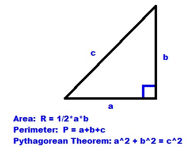
Problem:  Given the area of a right triangle (R) and perimeter (P), find the dimensions of the right triangle (a, b, and the hypotenuse c). 

Three facts about right triangles:

(I)  Area:  R = 1/2 * a * b
(II)  Perimeter:  P = a + b + c
(III) Pythagorean Theorem:  a^2 + b^2 = c^2

The task is to find a, b, and c:

Step 1:
Of (I): 
1/2 * a * b = R
a * b = 2 * R

Step 2:
Then from (II):
a + b + c = P
a + b = P – c

Step 3:
Squaring both sides:
(a + b)^2 = (P – c)^2

Step 4:
Expanding the left side:
a^2 + 2*a*b + b^2 = (P – c)^2
2*a*b + a^2 + b^2 = (P – c)^2

With a^2 + b^2 = c^2 (III) and a*b=2*R (Step 1):
2*(2*R) + c^2 = (P – c)^2

Simplify:
4*R + c^2 = P^2 – 2*P*c + c^2
4*R = P^2 – 2*P*c
c = (P^2 – 4*R)/(2*P)

Step 5: 
Rearrange (I) to solve for a (we could solve for b but the procedure is similar)
1/2 * a * b + R
a = (2*R)/b

Step 6: 
Use (III) and Step 5 to solve for b:
a + b + c = P
a + b = P – c
(2*R)/b + b = P – c
2*R + b^2 = b*(P – c)
(at this point, c is known)
b^2 – b*(P – c) + 2*R = 0

Using the quadratic formula:
b = ( (P-c) ± √((P-c)^2 – 8*R) )/2

In conclusion:
c = (P^2 – 4*R)/(2*P)
b = ( (P-c) ± √((P-c)^2 – 8*R) )/2
a = (2*R)/b = P – a - c

Example: 
Given R = 6 and P = 12

c = (12^2 – 4*6)/(2*12) = 5
b = ( (12-5) + √((12-5)^2 – 8*6) )/2 = 4
a = 12 – 5 – 4 = 3

c = (12^2 – 4*6)/(2*12) = 5
b = ( (12-5) - √((12-5)^2 – 8*6) )/2 = 3
a = 12 – 5 – 3 = 4

Solutions:
a = 3, b = 4, c = 5
or
a = 4, b = 3, c =5

Eddie


This blog is property of Edward Shore, 2016


Circles: Slope of the Line Segment from Point to Center vs. Slope of the Tangent Line

Circles:  Slope of the Line Segment from Point to Center vs. Slope of the Tangent Line


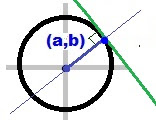
Consider a circle with point (a,b) on the circle.  Let’s compare the slopes of two lines:

(I) The line connecting the center of the circle and the point (a,b), and

(II) The slope of the tangent line containing point (a,b).  The tangent line is a line that touches the circle at point (a,b).

Case 1:  The center is (0, 0) (at the origin)

The equation of the circle is x^2 + y^2 = r^2, where r is the radius.

Since (a, b) is on the circle, then a^2 + b^2 = r^2. 

(I) Slope of the line connecting the center (0,0) and point (a,b).  Then the slope (labeled s1) is:

s1 = (b – 0)/(a – 0) = b/a

(II) Slope of the tangent line connecting (a,b).  The slope at point (a, b) would also be the slope of the tangent line.

Solving for y,

x^2 + y^2 = r^2
y^2 = r^2 – x^2
y = √(r^2 – x^2)

The derivative is:

dy/dx = 1/2 * (-2 * x) * (r^2 – x^2)^(-1/2)
dy/dx = -x / √(r^2 – x^2)

At point, (a, b), the slope (labeled s2) is:

s2 = -a / √(r^2 – a^2)

Since a^2 + b^2 = r^2,

s2 = -a / √(a^2 + b^2 – a^2)
s2 = -a / √(b^2)
s2 = -a/b

Note: Since s1 = b/a and s2 = -a/b, then s2 = -1/s1.

Case 2:  The is center is at point (m,n) with point (a,b) on the circle.

The equation of the circle becomes (x – m)^2 + (y – n)^2 = r^2. 
(I)  Slope of the line connecting the center (m, n) and point (a,b).  Then the slope (labeled s1) is:

s1 = (b –n)/(a – m)

(II) Slope of the tangent line connecting (a,b). 

Solving for y leads to:

(x – m)^2 + (y – n)^2 = r^2
(y – n)^2 = r^2 – (x -,m)^2
y = √(r^2 – (x – m)^2) + n

Taking the derivative:

dy/dx = -(x – m)/√(r^2 – (x-m)^2)

With the point (a,b):

s2 = -(a – m)/√(r^2 – (a – m)^2)
s2 = -(a – m)/√((a – m)^2 + (b – n)^2 – (a – m)^2)
s2 = -(a – m)/(b – n)

Since s1 = (b – n)/(a – m) and s2 = -(a – m)/(b – n), them s2 = -1/s1

Conclusion:  On a circle with center (m,n), with the point (a,b) on the circle, the slope of the tangent line through the point is –(a – m)/(b – n). 

Eddie

 This blog is property of Edward Shore, 2016.


Solving Absolute Value Equations

Solving Absolute Value Equations

Introduction

There are several ways to solve absolute value equations.  One way we can take advantage that |x|^2 = x^2, but only if we are dealing with real numbers.  To see why, please see the link below:


However, the surest way to solve equations involving absolute value equations.  Steps:

1.  Isolate the expression with absolute value one side of the equation. Hence to the equation to read something like this:  |f(x)| = g(x).
2.  Solve two equations:  f(x) = +g(x) and f(x) = -g(x).

Some examples of how the method works:


Example 1:

|x| + x = 5
|x| = 5 – x

The next step to solve two equations:  x = +(5 – x) and x = -(5 – x)

x = +(5 – x)
x = 5 – x
2x = 5
x = 5/2 

x = -(5 – x)
x= -5 + x
0 = -5, but 0 ≠ -5, so no solution in this case.

In our final analysis, x = 5/2

Example 2:

3*|x-2| = 6 + 4x
|x-2| = 2 + 4/3 * x

Now we need to solve both x – 2 = +(2 + 4/3*x) and x – 2 = -(2 + 4/3*x)

x – 2 = 2 + 4/3*x
-4 = 1/3 * x
-12 = x

x – 2 = -(2 + 4/3*x)
x – 2 = -2 – 4/3*x
0 = -7/3*x
0 = x

Both valid, so our solutions are x = -12 and x = 0.

Example 3:

|x^2 + 5*x + 6| = x

We know the drill, solve x^2 + 5*x + 6 = x and x^2 + 5*x + 6 = -x.

x^2 + 5*x + 6 = x
x^2 + 4*x + 6 = 0
x = (-4 ± √(16 – 24))/2
x = (-4 ± √(-8))/2
x = -2 ± i*√2

x^2 + 5*x + 6 = -x
x^2 + 6*x + 6 = 0
x = ( -6 ± √(36 – 24))/2
x = (-6 ± √12)/2
x = -3 ± √3

Hope you find this helpful, in the near future I want to tackle other common problems found in algebra. 

Eddie


This blog is property of Edward Shore, 2016.

HP Prime: Basic CAS Commands for Polynomials and Rational Expressions

HP Prime:  Basic CAS Commands for Polynomials and Rational Expressions


Define the following variables:

poly:  a polynomial of the form a_n*x^n + a_n-1*x^(n-1) + …. + a_1*x + a_0
rat:  a rational function consisting of the polynomials p(x)/q(x)
var: variable

Simplification Modes

Before we start, I want to comment on simplification modes.  

Simplification Modes:

None:  No simplification is executed
Minimum:  Simple simplification of results.  Additional simplification may be desired.
Maximum:  Full simplification of results

Below is a comparison between Minimum and Maximum modes.


To change Simplification mode, press [Shift], [CAS] (CAS Settings), and select a Simplification settings.  Select the Simplification drop down box and select the desired mode.    

Note:  The following examples are executed in Maximum simplification mode.

Part Extraction:  Coefficients, Numerator, Denominator

Coefficients

coef:  [Toolbox], (CAS), 6. Polynomial, 2.  Coefficients

Syntax:
coef(poly, var):  returns all the coefficients of a polynomial in a vector
coef(poly, var, n): return the coefficient of a polynomial in a vector of the specific power x^n

Examples:
coef(2x^2 + 3x – 1, x) returns [2, 3, -1]
coef(2x^2 + 3x – 1, x, 2) returns 2
coef(2x^2 + 3x – 1, x, 1) returns 3
coef(2x^2 + 3x – 1, x, 0) returns -1

Numerator and Denominator

numer: [Toolbox], (CAS), 1. Algebra, 8. Extract, 1.  Numerator
denom: [Toolbox], (CAS), 1. Algebra, 8. Extract, 2. Denominator

Syntax:
numer(rat)
denom(rat)

Example:
f≔(2x^2-3)/(x^2+1)
numer(f) returns 2*x^2 – 3
denom(f) returns x^2 + 1
purge(f) \\ this is to erase f

Polynomial Creation

Create a symbolic polynomial with a list of coefficients

poly2symb: [Toolbox], (CAS), 6. Polynomial, 7.  Create, 2. Coefs→Poly

Syntax:

poly2symb(vector of coefficients, var)

Example:

poly2symb( [8, -1, 0, 6], t) returns 8*t^3 – t^2 + 6

The inverse operation is the symb2poly(poly), which can be accessed by [Toolbox], (CAS), 6. Polynomial, 7. Create, 1. Poly→Create. 

Create a polynomial from a list of roots

This involves a two-step processes:
1. pcoeff( vector of roots )
2. poly2symb( result from step 1, var )

Access pcoeff: [Toolbox], (CAS), 6. Polynomial, 7. Create, 3.  Roots → Coef

You can combine the two steps by typing:  poly2symb(pcoeff( vector of roots), var).  Simplification may be required

Example:

pcoeff([-2, 5, 0, 6]) returns [1, -9, 8, 60, 0]
poly2symb([1, -9, 8, 60, 0],t) returns t^4 – 9*t^3 +8*t^2 + 60*t

poly2symb( pcoeff([2, -5, 0, 6]), t) returns 
t^4 – 9*t^3 + 8*t^2 + 60*t

Degree of a Polynomial

degree: [Toolbox], (CAS), 6, Polynomial, 8. Algebra, 3. Degree

Syntax:

degree(poly)

Example:
f: = 4*x^3 – 2*x^2 + 8*x – 8
degree(f) returns 3

You can factor a polynomial by x^n where n is the degree of the polynomial by using factor_xn.

factor_xn:  [Toolbox], (CAS), 6. Polynomial, 8. Algebra, 4. Factor By Degree
Caution:  This command works when the Simplification mode is turned to Minimum or Off.    

Example:
(after turning Simplification to Minimum)
factor_xn(f) returns x^3 * (4 – 2/x + 8/x^2 – 8/x^3)
purge(f)

Partial Fraction of Rational Functions

partfrac: [Toolbox], (CAS), 1. Algebra, 7. Partial Fraction

Syntax:

partfrac(rat)

Example:

partfrac( (x^4 – 3*x^3)/(x^2 -1) ) returns 
x^2 -3*x + 1 - 1/(x-1) - 2/(x+1)

Determining the Number of Zeros (Roots)

The sturmab command determines the number of zeros giving an interval.

sturmab:  [Toolbox], (CAS), 6. Polynomial, 8. Algebra, 6.  Zero Count

Syntax:

sturmab(poly, var, min, max)

The min and max can be complex numbers.

Examples:

sturmab(x^3 – 4*x^2 + 6*x – 4, x, -5, 5) returns 1  \\ 1 real root
sturmab(x^3 – 4*x^2 + 6*x – 4, x, -5-5*i, 5+5*i) returns 3  \\ 1 real, 2 complex roots

Polynomial Functions

Path: [Toolbox], (CAS), 6, Polynomial, 9. Special, then:
4.  Hermite \\ Syntax:  hermite(n)
7.  Legendre \\ Syntax:  legendre(n)
8.  Chebyshev Tn (1st Kind)  \\ Syntax:  tchebyshev1(n)
9.  Chebyshev Un (2nd Kind)  \\ Syntax:  tchebyshev2(n)

Where n is an integer.  You can specify a variable by adding var as a second argument. (x is the default variable)

Examples:
hermite(4) returns 16*x^4 – 48*x^2 + 12
legendre(4) returns (35*x^4 – 30*x^3 + 3)/8
tchebyshev1(4) returns 8*x^4 – 8*x^2 + 1
tchebyshev2(4) returns 16*x^4 – 12*x^2 + 1

This covers some of the basic CAS commands for polynomials and rational functions.  Hope you find this helpful,

Eddie


This blog is property of Edward Shore, 2016.


Wednesday, May 25, 2016

Android App Review: Matrix Calculator

Android App Review:  Matrix Calculator

Matrix Calculator
Platform:  Android
Author:  appassion.net
Version:  V 2.0.2, 4/21/2016
Price:  Free


This is a dedicated app to matrices.  It's as simple as that.  The operations available to you is dependent on the orientation of your device:

Portrait:  determinant (det), inverse (A^-1), transpose (A^T), matrix multiplication (*), clear
Landscape: det, A^-1, A^T, *, lower-upper decomposition (LU), matrix addition and subtraction

You can use the arrow keys to choose different elements in the matrix or create new rows and columns.  The other way is using the swiping motion. 

Matrices are automatically corrected. 

If you called an arithmetic operation (+, -, *), a new matrix is created.

I wish there was an easier way to delete elements, rows, and columns.  The only way to clear and delete elements is the repeated use of the [ C ] button.  If you were also expecting a scientific calculator with this app, then prepared to be disappointed.  This app is a single focus calculator, which is great if you work with matrices.  And you can’t beat the price.

Update (5/29/2016):  In a recent update, you can quickly clear entries and matrices by pressing and holding the clear key [C].  Thank you appassion.net!

This blog is property of Edward Shore, 2016.

Absolute Value: Does |x|^2 = x^2?

Absolute Value:  Does |x|^2 = x^2?

Proof that |x|^2 = x^2, assuming x is a real number.

Note that |x| = x/sgn(x), where sgn(x) is the sign function where:

sgn(x) = -1 if x < 0,
sgn(x) = 0 if x = 0,
and sgn(x) = 1 if x > 0

Case: x = 0. 

Then:
|0| = 0 and |0|^2 = 0^2 = 0.

Case: x ≠ 0.  

Then:
|x|^2 = (x/sgn(x))^2
= x/sgn(x) * x/sgn(x)
= x^2/sgn(x)^2

If x < 0, sgn(x) = -1, and since -1 * -1 = 1, sgn(x)^2 = 1
If x > 0, sgn(x) = 1, and since 1 * 1 = 1, sgn(x)^2 = 1

Hence:
x^2/sgn(x)^2
= x^2

QED

Caution:  The statement |x|^2 = x^2 is not true for complex numbers where the imaginary part is nonzero. 

Let x = a + b*i

|x|^2 = |a + b*i|^2 = (√(a^2 + b^2))^2 = a^2 + b^2

x^2 = (a + b*i)^2 = a^2 + 2*a*b*i – b^2 ≠ a^2 + b^2   (b ≠ 0)


Conclude:  |x|^2 = x^2 only if x is a real number.


Eddie


This blog is property of Edward Shore, 2016

Tuesday, May 24, 2016

TI-30Xa: Logarithm Bug Corrected (From Datamath Calculator Museum)

On top of Datamath's web page (http://www.datamath.org/,  Retrieved May 24, 2016), the website announced that a logarithm bug for several Texas Instruments has been addressed and corrected.  There is a big box on top the page which will you lead you to the article.  

This affects the basic level (one-line display) scientific calculators, from the TI-35X and TI-36X from the early 1990s to TI-30Xa of the 2010s.  The bug is present when you calculate the natural logarithm of numbers between 1.000000001 and 1.01.

Datamath reports that the bug has been fixed in 2015; hence the TI-30Xa and TI-30 ECO RS (the latter not in TI's United States product lineup) manufactured 2015 and after are working properly.


In testing the two TI-30Xa's I have (manufactured in 2011 and 2013, I think), it seems that they have the bug.  I might buy a new revision to test it.  


Update (5/25/2016):  I purchased a new TI-30xa today (manufacture number? L-0216M, the package had a date of 2015) to test whether the bug has been resolved.  I put this one and an older version (K-0513K – 2013) to the test.  To get the full decimal result, I put both calculators in scientific mode.  Judging by these results, the bug appears to have been resolved. 


A comparison between TI-30Xas.  The left is the 2016 (new) manufacture, the right is the 2013 (old) manufacture.  The results on the left are correct.  


Eddie

This blog is property of Edward Shore, 2016

Wednesday, May 18, 2016

Geometry: The Sagitta in Circles

Geometry:  The Sagitta in Circles

When the word Sagitta is mentioned, we would associate sagitta with a small constellation between the constellations Aquila and Cygnus.  Sagitta is one of the smallest constellations in astronomy.  In mythology, the Sagitta refers to an arrow, involved in a number of myths:  (1) the arrow Hercules used to kill an eagle to free Prometheus, (2) the arrow used by Apollo to avenge Asclepius’ death, and (3) the arrow Eros used to shoot Zeus to make him fall in love with Ganymede. 

But did you know that sagitta was referred to a length in geometry.  The sagitta is the length from the center of a circular arc to its base (defined by the circle’s chord). 


Variables: 
r = radius of the circle
c = chord length
s = sagitta
θ = angle between radius and line that connects center to end-chord line (see the diagram above)

Derivation:  Calculating the length of the sagitta

Given radius and angle:

cos θ = (r – s) / r
r * cos θ = r – s
s = r – r cos θ
s = r * (1 – cos θ)

Example:  r = 5, θ = 60°

s = 5 * (1 – cos 60°)
s = 2.5

Given radius and chord length:

(r – s)^2 + (c/2)^2 = r^2
(r – s)^2 = r^2 – (c/2)^2
r – s = √(r^2 – (c/2)^2)
s = r - √(r^2 – (c/2)^2)

Example:  c = 10, r = 6

s = 6 - √(6^2 – (10/2)^2)
s ≈ 2.68338

Sources:

“Sagitta (geometry)”.  Wikipedia.  https://en.wikipedia.org/wiki/Sagitta_(geometry)  Retrieved May 6, 2016

“Sagitta Constellation”  Constellation Guide.  Constellations:  A Guide to the Night Sky  http://www.constellation-guide.com/constellation-list/sagitta-constellation/   Retrieved May 18, 2016


This blog is property of Edward Shore, 2016.

Tuesday, May 17, 2016

HP Prime: Algebraic CAS Commands

HP Prime:  Algebraic CAS Commands

On today’s entry I am going discuss several CAS (Computer Algebraic System) commands: factor, expand, collect, and subst (substitute).   These four commands are common to calculators, mathematical software, and mathematical apps that have CAS commands.

If you have not heard about CAS before, CAS allows the user to operate on expressions with indefinite (undefined) variables.  CAS commands commonly manipulate algebraic expressions, calculate derivatives of functions, and calculate indefinite integrals.    My first experience with CAS commands was with the (original) TI-89 almost a decade and half ago.  (Wow, I’m getting old).  Let’s get started. 

On the HP Prime, you can enter CAS mode by pressing the [CAS] button. In CAS mode, the variables are primarily lower case.  Single letter uppercase variables, along with θ, are always numeric. 

Note:  Radian mode is used.

Factor

Two type of factoring functions:  factor and ifactors.

factor:  [Toolbox], (CAS), 1. Algebra, 4. Factor

The command factor works with polynomials and rational expressions. 

Examples: 
factor(x^2 + 6*x + 5) returns (x + 1)*(x + 5)
factor(x^2 + x – 4) returns (x + (1 - √17) / 2) * (x + (1 + √17) / 2)
factor(x^2 + 4*x + 4) returns (x + 2)^2

TIP:  If you are not sure whether implied multiplication will be accepted, insert the multiply operators (*) in the expression.  It is always a safe bet. 

ifactors:  [Toolbox], (CAS), 5.  Integer, 2. Factors

Unlike factor, ifactors works on factoring integers into their prime factorizations.  If the integer is prime, the integer itself is returned. 

Examples:
ifactors(55) returns 5 * 11
ifactors(2162) returns 2 * 23 * 47
ifactors(1367) returns 1367   (1367 is prime)

Expand

There are three expand commands we’ll cover:  expand, powexpand, and texpand.  Which command that you use determines what time of expression to be expanded. 

expand:  [Toolbox], (CAS), 1.  Algebra, 4.  Factor

The command expand works on polynomials and rational functions.  It can be thought of that expand is the opposite of factor. 

Examples:
expand( (x - 1)^3 ) returns x^3 – 3*x^2 + 3*x - 1
expand( (x + 1)^2 * (x^2 – 3) ) returns x^4 + 2*x^3 – 2*x^2 – 6*x – 3

powexpand:  [Toolbox], (CAS), 4.  Rewrite, 2.  powexpand

The command powexpand involves expressions with exponents. 

powexpand( x^(2 + a) ) returns x^2 * x^a

Sometimes you have to combine one or more CAS commands to get what you want. 

powexpand( x^((a + 1) * (a + 5)) ) returns x^((a + 1) * (a + 5)).   

This is not a result I would want.  Let’s tackle this another way: 

expand( (a + 1)*(a + 5) ) returns a^2 + 6*a + 5, then
powexpand( x^(a^2 + 6*a + 5) ) returns x^a^2 * (x^a)^6 * x^5

texpand:  [Toolbox], (CAS), 4. Rewrite, 3. Texapnd

The command texpand is part of the expand family, this time texpand works with transcendental functions (sin, cos, tan, ln, exp). 

texpand( sin(2*x) ) returns 2 * cos(x) * sin(x)
texpand( cos (2*x + 1) ) returns (2 * cos(x)^2 – 1) * cos(1) – 2 * cos(x) * sin(x) * sin(1)
texpand( e^(3*x) + cos(3*x) ) returns e^x^3 + 4 * cos(x)^3 – 3 * cos(x)

Collect

collect:  [Toolbox], (CAS), 1.  Algebra, 2.  Collect

This commands collects like terms in a polynomial, and when applicable factorizes the expressions.  The variable to collect around may be specified.

Examples:

collect( (x + 1)^2 + x^2 + 2*x ) returns 2*x^2 + 4*x + 1

collect( (x + a + 2*(x + a) ) returns 3 * (a + x)
collect( (x + a + 2*(x + a), a ) returns 3*a + 3*x
collect( (x + a + 2*(x + a), x ) returns 3*a + 3*x

collect( (x^2 + a^2 + 2*(x + a)^2 ) returns 4*a*x + 3*a^2 + 3*x^2
collect( (x^2 + a^2 + 2*(x + a)^2, a ) returns a * (3*a + 4*x) + 3*x^2
collect( (x^2 + a^2 + 2*(x + a)^2, x ) returns x * (4*a + 3*x) + 3*a^2

Substitute

This does exactly what it is says:  substitute.  
Syntax:  subst(expression, var = value/expr)

subst:  [Toolbox], (CAS), 1. Algebra, 6. Substitute

Examples:

subst( x^4 + 2*x^2 – x, x = √a) returns a^2 + 2*a - √a

Here are two examples where an additional CAS command is needed to simplify:

subst( cos(2*x), x = asin(a) ) returns cos( 2* asin(a) )
texpand(cos( 2* asin(a) ) returns 2*(1 – a^2) – 1

subst( 2*x^2 – x, x = a + 3 ) returns 2*(a + 3)^2 – a – 3
expand(2*(a + 3)^2 – a – 3 ) returns 2*a^2 + 11*a + 15

There are four common CAS commands, I hope you find this helpful.

Eddie

This blog is property of Edward Shore, 2016.


Sunday, May 15, 2016

Fraction Approximation on Graphing Calculators Comparisons

Fraction Approximation on Graphing Calculators Comparisons

 Advanced calculators and calculator apps sometimes give the ability for the user to convert answers to fractions.  For rational numbers, the fractional conversions are precise and easy.  However, for irrational numbers, different calculators use different algorithms.  I am going to use three calculators to compare fractional answers:

TI-Nspire CAS iOS App:  Fractional Approximations

* TI-NSpire CAS iOS App:  this should be similar to the TI-Nspire CAS handheld calculators, x→approxFraction(5.E-14)

* Casio Classpad fx-CP400:  fractional approximation used by tofrac(approx(x))

* HP Prime (firmware 10077), pressing [a b/c] after the number is entered

Square Root of 2, √2
Decimal Approximation
1.41421356237
TI-NSpire CAS
3,880,899/2,744,210
Casio Classpad fx-CP400
13,250,218/9,369,319
HP Prime
114,243/80,782

Square Root of 3, √3
Approximation
1.73205080757
TI-NSpire CAS
3,650,401/2,107,560
Casio Classpad fx-CP400
3,650,401/2,107,560
HP Prime
191,861/110,771

Square Root of 5, √5
Approximation
2.2360679775
TI-NSpire CAS
3,940,598/1,762,289
Casio Classpad fx-CP400
16,692,641/7,465,176
HP Prime
219,602/98,209

Euler’s Number, e
Approximation
2.71828182846
TI-NSpire CAS
14,665,106/5,394,991
Casio Classpad fx-CP400
14,665,106/5,394,991
HP Prime
219,602/98,209

The Constant Pi, π
Approximation
3.14159265359
TI-NSpire CAS
5,149,351/1,725,033
Casio Classpad fx-CP400
69,305,155/22,060,516
HP Prime
312,689/99,532

The Constant Pi, π^2
Approximation
9.86960440109
TI-NSpire CAS
26,140,802/2,648,617
Casio Classpad fx-CP400
26,140,802/2,648,617
HP Prime
12,59,401/127,604

The Golden Ratio, Φ = (1 + √5)/2
Approximation
1.61803398875
TI-NSpire CAS
5,702,887/3,524,578
Casio Classpad fx-CP400
5,702,887/3,524,578
HP Prime
121,393/75,025

The Zeta of 3, ζ(3) ≈ 1.20205693015959428539
Approximation
1.20205690316
TI-NSpire CAS
2,721,755/2,264,248
Casio Classpad fx-CP400
2,721,755/2,264,248
HP Prime
927,328/771,451


This blog is property of Edward Shore, 2016

Numworks: Allowing Repeated Calculations in Python

Numworks: Allowing Repeated Calculations in Python Introduction Say we want the user to repeat a calculation or a routine for as lo...