Thursday, March 31, 2022

March Calculus Madness Sweet Sixteen - Day 16: A Parametric Integral Example

 ------------


Welcome to March Calculus Madness!


------------


Let:

x(t) = a * cos t

y(t) = b * sin t


Then:

∫ y(x) dx = ∫ y(t) * x'(t) dt


x'(t) = -a * sin t


And:

∫ y(t) * x'(t) dt

= ∫ -a * sin t * b * sin t dt

= -a * b * ∫ sin^2 t dt

= -a * b * ∫1/2 - 1/2 * cos(2*t) dt

= -a * b * (t/2 - sin(2*t)/4) + C


That wraps up March Calculus Madness 2022.  


Next Post:  April 9, 2022


Have a great day and hope you enjoyed the series!  


Eddie 


All original content copyright, © 2011-2022.  Edward Shore.   Unauthorized use and/or unauthorized distribution for commercial purposes without express and written permission from the author is strictly prohibited.  This blog entry may be distributed for noncommercial purposes, provided that full credit is given to the author. 


Wednesday, March 30, 2022

March Calculus Madness Sweet Sixteen - Day 15: r = α * (1 - cos Θ)

 ------------


Welcome to March Calculus Madness!


------------


r = α * (1 - cos Θ)


r = α * (1 - cos Θ)

r^2 = α^2 * (1 - 2 * cos Θ + cos^2 Θ)


dr/dΘ = α * sin Θ

(dr/dΘ)^2 = α^2 * sin^2 Θ


Area from 0 ≤ Θ ≤ 2*π


1/2 * ∫ α^2 * (1 - cos Θ)^2  dΘ from Θ = 0 to Θ = 2*π

= α^2/2 * ∫ 1 - 2 * cos Θ + cos^2 Θ dΘ from Θ = 0 to Θ = 2*π

= α^2/2 * ∫ 1 - 2 * cos Θ + 1/2 * cos(2*Θ) + 1/2 dΘ from Θ = 0 to Θ = 2*π

= α^2/2 * (3/2 * Θ - 2 * sin Θ + 1/4 * sin(2*Θ) from Θ = 0 to Θ = 2*π)

= 3/2 * π * α^2


Arc Length from 0 ≤ Θ ≤ 2*π


r^2 + (dr/dΘ)^2

= α^2 * (1 - 2 * cos Θ + cos^2 Θ) + α^2 * sin^2 Θ

= α^2 - 2  * α^2 * cos Θ + α^2 * (cos^2 Θ + sin^2 Θ)

= α^2 - 2  * α^2 * cos Θ + α^2 

= 2 * α^2 - 2 * α^2 * cos Θ

= 2 * α^2 *(1  - cos Θ)


Arc Length:

∫ 2 * α^2 *(1  - cos Θ) dΘ from Θ = 0 to Θ = 2*π

= α * √2 * ∫ √(1  cos Θ) dΘ from Θ = 0 to Θ = 2*π

= α * √2 * 4 * √2

= 8 * α


Eddie 


All original content copyright, © 2011-2022.  Edward Shore.   Unauthorized use and/or unauthorized distribution for commercial purposes without express and written permission from the author is strictly prohibited.  This blog entry may be distributed for noncommercial purposes, provided that full credit is given to the author. 


Tuesday, March 29, 2022

March Calculus Madness Sweet Sixteen - Day 14: The Arc Length of a Spiral

 ------------


Welcome to March Calculus Madness!


------------


The Length of a Spiral from 0 ≤ Θ ≤ m


The equation of a spiral:  r = α * Θ


The arc length of a polar equation r(Θ):  ∫ √(r(Θ)^2 + (dr/dΘ)^2) dΘ


r = α * Θ

r^2 = α^2 * Θ^2


dr = α dΘ

(dr/dΘ)^2 = α^2


∫ √(α^2 * Θ^2 + α^2) dΘ from Θ = 0 to Θ = m

= α * ∫ √(Θ^2 + 1) dΘ from Θ = 0 to Θ = m

= α/2 * ( ln|Θ + √(1 + Θ^2)| + Θ * √(1 + Θ^2) for Θ = 0 to Θ = m)

(see below)

= α/2 * ( ln|m + √(1 + m^2)| + m * √(1 + m^2) )


Aside:

∫ √(1 + Θ^2) dΘ


Let Θ = tan x

dΘ = sec^2 x dx


∫ √(1 + Θ^2) dΘ

= ∫ √(1 + tan^2 x) * sec^2 x  dx

= ∫ √(sec^2 x) * sec^2 x dx

= ∫ sec^3 x dx

= 1/2 * ∫ sec x dx + (sec x * tan x)/2 + C

(per reduction integration rule for sec x)


= 1/2 * ln|tan x + sec x| + 1/2 * sec x * tan x + C


with: 

Θ = tan x

arctan Θ = x

sec(arctan Θ) = sec x

√(1 + x^2) = sec x


= 1/2 * ln|Θ + √(1 + Θ^2)| + 1/2 * Θ * √(1 + Θ^2) + C


Eddie 


All original content copyright, © 2011-2022.  Edward Shore.   Unauthorized use and/or unauthorized distribution for commercial purposes without express and written permission from the author is strictly prohibited.  This blog entry may be distributed for noncommercial purposes, provided that full credit is given to the author. 


Monday, March 28, 2022

Retro Review: TI Investment Analyst

 Retro Review:   TI Investment Analyst


Today's review will be on a specialized calculator that had a very short life in the market:  the Texas Instruments Investment Analyst.  


Quick Facts:


Model:  Investment Analyst

Company:  Texas Instruments

Years:  1979-1980

Type:  Specialized Finance

Batteries: 2 x LR44

Operating Mode:  Chain


Features: Stocks, Bonds, Options


*  The [CIF] key:  which calculates (1 + i%)^n.  Used in time value of money calculations.


* Days between Dates allowing for four digit years.  The manual states that this function is accurate for the range March 1, 1900 to February 28, 2100.  The date format is mmdd.yyyy.  Example:  March 28, 2022 is 328.2022.


* The [ 2nd ] (Sec Typ) sets the security type mode.  


Stocks (Security Type A)  


We can solve for the purchase price (buy), selling price (sell), and yield.   Variables include:


**  the number of days until the first dividend is paid (B→P), the number of days from 

**  the last dividend until the stock is sold (P←S)

**  capital gains tax rate and income tax rate 

**  commissions rate when the stock is bought and sold

**  dividends, and dividend growth rate


**  The Investment Analyst has two modes for stocks:  annual yield and ownership period yield.  The latter mode is simpler.  


Bonds (Security Type B)


The keys to operate calculations for bonds are the mostly the same set of keys used for stocks.  We still solve for price (buy), selling price (sell), and yield. 


**  Annual yield mode is automatic

**  payments during investments are now coupons, which the coupon rate is entered with the [ CPN ] key

**  commissions, capital gains tax rate, and income tax rate are still included


I do believe that bonds make it into later calculators, such as the TI BA II Plus.   


Options (Security Type is "Blank")


Generally the same concept, solve for price (buy), selling price (sell), and yield; with variables including commissions, capital gains tax, and income tax.   What is different is the use of call and put prices.  


I realize that this is a short introduction, as I plan to learn more about the features of the Investment Analyst.  


Keyboard


The keys are little hard, careful pressing of them are required. I find this to be the case of TI's calculators from the late 1970s/early 1980s. Thankfully the keyboard is still workable.  


I wonder if the keyboards were lot better, calculators outside of the "mainstream" such as the Investment Analyst and the TI-54 (which I reviewed in 2018) would have been given another edition.  


Closing Thoughts


This is a curious calculator that fit a specialized niche: stocks, bonds, and options.   Not too many calculators go into this area, I believe Calculated Industries had one dedicated to Wall Street calculations.  I have a feeling I am going to learn a lot about investments from going through the well detailed manual.  


This is definitely a collector's item.  


Source:

"Texas Instruments Investment Analyst"  Datamath Calculator Museum.  December 5, 2001.  Last retrieved March 4, 2022.    http://www.datamath.org/Sci/Slimline/Investment-Analyst.htm   


Until next time,


Eddie


All original content copyright, © 2011-2022.  Edward Shore.   Unauthorized use and/or unauthorized distribution for commercial purposes without express and written permission from the author is strictly prohibited.  This blog entry may be distributed for noncommercial purposes, provided that full credit is given to the author. 


March Calculus Madness Sweet Sixteen - Day 13: Some Double Integrals

 ------------


Welcome to March Calculus Madness!


------------


Double Integration Time


(I) 

∫ ∫ sin(a*x + b*y) dx dy

= ∫ -1/a * cos(a*x + b*y) + C1 dy

= -1/(a*b) * sin(a*x + b*y) + C1*y + C2


(II) 

∫ ∫ sin(a*x + b*y) dy dx

= ∫ -1/b * cos(a*x + b*y)+ C1 dx

= -1/(a*b) * sin(a*x + b*y) + C1 * x + C2


For (I) and (II) to equal,  x = y


(III)

∫ ∫ e^(a*x + b*y) dx dy

= ∫ 1/a * e^(a*x + b*y)+ C1 dy

= 1/(a*b) * e^(a*x + b*y) + C1 * y + C2


(IV)

∫ ∫ e^(a*x + b*y) dy dx

= ∫ 1/b * e^(a*x + b*y) + C1  dx

= 1/(a*b) * e^(a*x + b*y) + C1 * x + C2


For (III) and (IV) to be equal, x = y


Eddie


All original content copyright, © 2011-2022.  Edward Shore.   Unauthorized use and/or unauthorized distribution for commercial purposes without express and written permission from the author is strictly prohibited.  This blog entry may be distributed for noncommercial purposes, provided that full credit is given to the author. 


Sunday, March 27, 2022

March Calculus Madness Sweet Sixteen - Day 12: Arc Length of Sine and Cosine

 ------------


Welcome to March Calculus Madness!


------------


What is the arc length of y = sin x and y = cos x from x = 0 to x = 2 * π


The arc length of y(x) is calculated by:


∫ √(1 + (dy/dx)^2) dx for x = a to x = b


For y(x) = sin x, dy/dx = cos x, (dy/dx)^2 = cos^2 x


Arc length of y = sin x from x = 0 to x = 2*π

∫ √(1 + cos^2 x) dx for x = 0 to x = 2*π ≈ 7.64039557806


Likewise, for y(x) = cos x, dy/dx = -sin x, (dy/dx)^2 = sin^2 x

∫ √(1 + sin^2 x) dx for x = 0 to x = 2*π ≈ 7.64039557806


Yes, the arc lengths are the approximately the same.  


Eddie


All original content copyright, © 2011-2022.  Edward Shore.   Unauthorized use and/or unauthorized distribution for commercial purposes without express and written permission from the author is strictly prohibited.  This blog entry may be distributed for noncommercial purposes, provided that full credit is given to the author. 


Saturday, March 26, 2022

March Calculus Madness Sweet Sixteen - Day 11: ∫ int(x) dx

 ------------


Welcome to March Calculus Madness!


------------


f(x) = IP(x), integer function, HP Prime


int(x):  integer part function


Domain:

0 ≤ x < 1;  int(x) = 0

1 ≤ x < 2;  int(x) = 1

2 ≤ x < 3;  int(x) = 2

3 ≤ x < 4;  int(x) = 3


Hence:


∫ int(x) dx for x = 1 to x = 2 

= lim a→2- ∫ 1 dx for x = 1 to x = a

= lim a→2-  a - 1

= 2 - 1

= 1


∫ int(x) dx for x = 2 to x = 3 

= lim a→3- ∫ 1 dx for x = 1 to x = a

= lim a→3-  2 * a - 2 * 2

= 2 * 3 - 4 

= 2


∫ int(x) dx for x = 3 to 4 

= lim a→4- ∫ 1 dx for x = 1 to a

= lim a→4-  3 * a - 3 * 3 

= 4 * 3 - 9

= 3


and so on...


∫ int(x) dx for x = 1 to x =3 

= (∫ int(x) dx for x =1 to x=2 )+ (∫ int(x) dx for x =2 to x=3) + (∫ int(x) dx for x=3 to x=4 )

= 1 + 2 + 3

= 6


The General Integral ∫ int(x) dx for x = 1 to x = t


∫ int(x) dx for x = 1 to x = t

= ∫ int(x) dx for x = 1 to x = int(t) + ∫ int(x) dx for x = int(t) to x = t

= lim a→int(t)- ∫ int(x) dx for x = 1 to x = a + ∫ int(x) dx for x = int(t) to x = t

= (1 + 2 + 3 + 4 + .... + t-1) + t * int(t) - int(t) * int(t)

= t * (t-1)/2 + t * int(t) - int^2(t)


Example:


∫ int(x) dx for x = 1 to x = 8.3

= (7 * 8)2 + (8.3 * 8 - 8^2)

= 30.4


Eddie 


All original content copyright, © 2011-2022.  Edward Shore.   Unauthorized use and/or unauthorized distribution for commercial purposes without express and written permission from the author is strictly prohibited.  This blog entry may be distributed for noncommercial purposes, provided that full credit is given to the author. 


Friday, March 25, 2022

March Calculus Madness Sweet Sixteen - Day 10: ∫ frac(x) dx

 ------------


Welcome to March Calculus Madness!


------------


frac(x) - HP Prime


frac(x):  fractional part function


Domain:  0 ≤ frac(x) < 1


∫ frac(x) dx for x = 0 to 1


According to the graph above, the area between resembles as a right triangle.


When 0≤x<1, frac(x) = x


Hence:

∫ frac(x) dx for x = 0 to x = 1


Note:  

lim a→1-  (∫ frac(x) dx for x = 0 to x = a)

= lim a→1-  (∫ x dx for x = 0 to x = a)

= lim a→1-  (∫ x dx for x = 0 to x = a)

= lim a→1-  (a^2/2 - 0)

= 1/2


What if the upper limit is less than 1? 


Let b where, 0≤x≤b<1  (b<1):


∫ frac(x) dx for x = 0 to x = b

= ∫ x dx for x = 0 to x = b

= b^2/2


Eddie 


All original content copyright, © 2011-2022.  Edward Shore.   Unauthorized use and/or unauthorized distribution for commercial purposes without express and written permission from the author is strictly prohibited.  This blog entry may be distributed for noncommercial purposes, provided that full credit is given to the author. 


Thursday, March 24, 2022

March Calculus Madness Sweet Sixteen - Day 9: ∫ e^x/(e^x + 1) dx and ∫ e^x/(e^x - 1) dx

 ------------


Welcome to March Calculus Madness!


------------


∫ e^x/(e^x + 1) dx


Let z = e^x

Then: 

ln z = x

1/z dz = dx


∫ e^x/(e^x + 1) dx

= ∫ z/(z + 1) * 1/z dz

= ∫ 1/(z + 1) dz

= ln |z + 1| + C

= ln |e^x + 1| + C


∫ e^x/(e^x - 1) dx


Again, let z = e^x


∫ e^x/(e^x - 1) dx

= ∫ z/(z - 1) * 1/z dz

= ∫ 1/(z - 1) dz

= ln |z - 1| + C

= ln |e^x - 1| + C


Eddie 


All original content copyright, © 2011-2022.  Edward Shore.   Unauthorized use and/or unauthorized distribution for commercial purposes without express and written permission from the author is strictly prohibited.  This blog entry may be distributed for noncommercial purposes, provided that full credit is given to the author. 


Wednesday, March 23, 2022

March Calculus Madness Sweet Sixteen - Day 8: ∫ ln^2 x dx and ∫ ln^3 x dx

 ------------


Welcome to March Calculus Madness!


------------


Integration by parts to the rescue!


∫ ln^2 x dx


u = ln^2 x,   dv = dx

du = 2 * ln * 1/x dx,   v = x


∫ ln^2 x dx

= x * ln^2 x - ∫ 2 * ln x * 1/x * x dx

= x * ln^2 x - ∫ 2 * ln x dx


u = ln x, dv = 2 dx

du = 1/x dx, v = 2 * x


= x * ln^2 x - (2 * x * ln x - ∫ 1/x * 2 * x dx)

= x * ln^2 x - (2 * x * ln x - ∫ 2 dx)

= x * ln^2 x - 2 * x * ln x + ∫ 2 dx

= x * ln^2 x - 2 * x * ln x + 2 * x + C


∫ ln^3 x dx


u = ln^3 x dx, dv = dx

du = 3 * ln^2 x dx, v = x


= x * ln^3 x - ∫3 * ln^2 x * 1/x * x dx

= x * ln^3 x - 3 * ∫ ln^2 x dx

= x * ln^3 x - 3 * (x * ln^2 x - 2 * x * ln x + 2 * x + C)

(see the above)

=  x * ln^3 x - 3 * x * ln^2 x + 6 * x * ln x - 6 * x + D   

(where D = 3 * C, C and D are constants)


Eddie


All original content copyright, © 2011-2022.  Edward Shore.   Unauthorized use and/or unauthorized distribution for commercial purposes without express and written permission from the author is strictly prohibited.  This blog entry may be distributed for noncommercial purposes, provided that full credit is given to the author. 


Tuesday, March 22, 2022

March Calculus Madness Sweet Sixteen - Day 7: ∫ 1/(1 + cos x) dx and ∫ 1/(1 + sin x) dx

 ------------


Welcome to March Calculus Madness!


------------


∫ 1/(1 + cos x) dx and ∫ 1/(1 + sin x) dx


To tackle these integrals, we will make use of the following derivatives and trig identities:


d/dx tan x = sec^2 x dx


d/dx cot x = -csc^2 x dx


d/dx csc x = -cot x * csc x


d/dx sec x = tan x * sec x


sin^2 x + cos^2 x = 1


cot x = 1/tan x,  csc x = 1/sin x,  sec x = 1/cos x


∫ 1/(1 + cos x) dx

= ∫ 1/(1 + cos x) * (1 - cos x)/(1 - cos x) dx

= ∫ (1 - cos x)/(1 - cos^2 x) dx

= ∫ (1 - cos x)/sin^2 x dx

= ∫ csc^2 x - cot x * csc x dx

= -cot x + csc x + C


∫ 1/(1 + sin x) dx

= ∫ 1/(1 + sin x) * (1 - sin x)/(1 - sin^2 x) dx

= ∫ (1 - sin x)/(1 - sin^2 x) dx

= ∫ (1 - sin x)/(cos^2 x) dx

= ∫ sec^2 x - tan x * sec x dx

= tan x - sec x + C


Note:  CAS systems in graphing calculators will default to using sin x, cos x, and tan x.  


Eddie


All original content copyright, © 2011-2022.  Edward Shore.   Unauthorized use and/or unauthorized distribution for commercial purposes without express and written permission from the author is strictly prohibited.  This blog entry may be distributed for noncommercial purposes, provided that full credit is given to the author. 

Monday, March 21, 2022

Swiss Micros DM42/HP42S: Polynomial Solver

 Swiss Micros DM42/HP42S:  Polynomial Solver


Introduction


The solver PSOL (pmatsolver.raw) uses a two column matrix PMAT to evaluate and solve for polynomials in the form:


p(x) = a1 * x^b1 + a2 * x^b2 + a3 * x^b3 + ...


And PMAT has the matrix in the form of:


[ [ a1,  b1 ],  

[ a2, b2 ], 

[ a3, b3 ] ... ]


The PMAT Matrix


The solver uses the matrix PMAT.  It must first be created in order for the solver to work.


Creating PMAT:    

1.  Enter the number of terms, press [ENTER], type 2, press [(shift)] [ 9 ] (MATRIX), select (NEW).

2.  Select (EDIT) from the MATRIX menu.

3.  Enter the coefficients and powers.   For terms in form of a1, the power is 0.  For terms in form of x^b1, the coefficient is 1.

4.  Press [EXIT], then [STO], [(shift)] [ENTER] (ALPHA), type PMAT.


Editing PMAT:

1.  Enter the number of terms, press [ENTER], type 2, press [(shift)] [ 9 ] (MATRIX), select (DIM), select PMAT.

2.  From the MATRIX menu, select (EDITN), select PMAT.  Be sure to select EDITN (edit named matrix).


Running the Solver


To run the polynomial solver:

1.  Press [(shift)] [ 7 ] (SOLVER), select PSOL.

2.  To evaluate p(x), enter a value for X and solve for P.   

3.  To solve for x, enter a value for P, enter a guess for X, and then press X again to solve.


Note:  The solver cannot evaluate 0^0.  Hopefully you can see why in the program listing.


The best part of PSOL is that you don't have to use just integer powers, put powers in order, or fill in zero terms (0 * x^n).


Examples


Example 1:  p(x) = 2 + 3x^1.5 - x^3


Set PMAT to be this:

[ [ 2, 0 ], 

[ 3, 1.5 ]

[ -1, 3 ] ]


If X = 2.2, solving for P yields 1.141382003

If P = -1, solving for X with guess 0 yields 2.431407988


Example 2:  p(x) = -5 + 3*x + 4*x^2


Set PMAT to be this:

[ [ -5, 0 ],

[ 3, 1 ], 

[ 4, 2 ]]


If X =1.8, solving for P yields 13.36

If P = 10, solving for X with guess 0 yields 1.59746673 


DM42/HP42S (Free42) Solver Program PSOL


00 { 65-Byte Prgm }

01 LBL "PSOL"

02 MVAR "P"

03 MVAR "X"

04 0

05 STO 01

06 INDEX "PMAT"

07 RCL "PMAT"

08 DIM?

09 R↓

10 STO 02

11 LBL 00

12 RCLEL

13 RCL "X"

14 J+

15 RCLEL

16 Y↑X

17 ×

18 STO+ 01

19 RCLIJ

20 R↓

21 RCL 02

22 X=Y?

23 GTO 01

24 J-

25 I+

26 GTO 00

27 LBL 01

28 RCL 01

29 RCL- "P"

30 .END.


Eddie


All original content copyright, © 2011-2022.  Edward Shore.   Unauthorized use and/or unauthorized distribution for commercial purposes without express and written permission from the author is strictly prohibited.  This blog entry may be distributed for noncommercial purposes, provided that full credit is given to the author. 


March Calculus Madness Sweet Sixteen - Day 6: ∫ √a ÷ (√(x+a) - √x) dx

 ------------


Welcome to March Calculus Madness!


------------


∫ √a ÷ (√(x+a) - √x) dx


Simplify:

√a ÷ (√(x+a) - √x)


Multiply by (√(x+a) + √x) ÷ (√(x+a) + √x) 


√a ÷ (√(x+a) - √x)

= √a ÷ (√(x+a) - √x) * (√(x+a) + √x) ÷ (√(x+a) + √x) 

= √a * (√(x+a) + √x) ÷ (x + a - x)

= 1 ÷ √a * (√(x+a) + √x)


Then:

∫ √a ÷ (√(x+a) + √x) dx

=  ∫ 1 ÷ √a * (√(x+a) + √x) dx

= a^(-1/2) * ∫ (x+a)^(1/2) + x^(1/2) dx

= 2 ÷ (3 * a^(1/2)) * ((x + a)^(3/2) + x^(3/2)) + C

= 2 ÷ (3 * a^0.5) * ((x + a)^1.5 + x^1.5) + C


Questions of preference:


Which is your preferred notation:


(1)  √x,  x^(1/2), or x^0.5?


(2)  x^(3/2) or x^1.5?  


Let us know in the comments.


Eddie 


All original content copyright, © 2011-2022.  Edward Shore.   Unauthorized use and/or unauthorized distribution for commercial purposes without express and written permission from the author is strictly prohibited.  This blog entry may be distributed for noncommercial purposes, provided that full credit is given to the author. 


Sunday, March 20, 2022

March Calculus Madness Sweet Sixteen - Day 5: x^n ∙ √(1 + x)

 ------------


Welcome to March Calculus Madness!


------------


d/dx x^n ∙ √(1 + x)


Here we can make use the multiplication rule:

d/dx f(x) ∙ g(x) = f(x) ∙ g'(x) + f'(x) ∙ g(x)


In this case:

f(x) = x^n

g(x) = √(1 + x) = (1 + x)^(1/2)


Then:

f'(x) = n ∙ x^(n-1)

g'(x) = 1/2 ∙ (1 + x)^(-1/2)


And: 

d/dx x^n ∙ √(1 + x) 

= x^n ∙ 1/2 ∙ (1 + x)^(-1/2) + n ∙ x^(n-1) ∙ (1 + x)^(1/2)


For indefinite integrals, I will do two specific cases of n.


∫ x ∙ √(1 + x) dx   (n = 1)


Using integration by parts:


u = x,  dv = (1 + x)^(1/2) dx

du = dx,  v = 2/3 ∙ (1+x)^(3/2)


∫ x ∙ √(1 + x) dx

= 2/3 ∙ (1+x)^(3/2) ∙ x - ∫ (1 + x)^(1/2) dx

= 2/3 ∙ (1+x)^(3/2) ∙ x - 2/3 ∙ (1 + x)^(3/2) + C

= 2/3 ∙ (1 + x)^(3/2) ∙ (x - 1) + C


∫ x^2 ∙ √(1 + x) dx   (n = 2)


Let z = (1 + x)^(1/2)

dz = 1/2 ∙ (1+ x)^(-1/2) dx

2 ∙ (1+x)^(1/2) dz = dx

2 ∙ z  dz = dx


z^2 = 1 + x

z^2 - 1 = x

z^4 - 2 ∙ z^2 + 1 = x^2


∫ x^2 ∙ √(1 + x) dx   

= ∫ (z^4 - 2 ∙ z^2 + 1) ∙ z ∙ 2 ∙ z dz

= ∫ (z^4 - 2 ∙ z^2 + 1) ∙ 2 ∙ z^2 dz

= ∫ 2 ∙ z^6 - 4 ∙ z^4 + 2 ∙ z^2 dz

= 2/7 ∙ z^7 - 4/5 ∙ z^5 + 2/3 ∙ z^3 + C

= 2/7 ∙ (1 + x)^(7/2) - 4/5 ∙ (1 + x)^(5/2) + 2/3 ∙ (1 + x)^(3/2) + C

(z = (1 + x)^(1/2))


Eddie


All original content copyright, © 2011-2022.  Edward Shore.   Unauthorized use and/or unauthorized distribution for commercial purposes without express and written permission from the author is strictly prohibited.  This blog entry may be distributed for noncommercial purposes, provided that full credit is given to the author. 


Saturday, March 19, 2022

March Calculus Madness Sweet Sixteen - Day 4: ∫x^2 / √(1 - x^2) dx

 ------------


Welcome to March Calculus Madness!


------------


∫x^2 / √(1 - x^2)  dx


Substitute:  z = arcsin x


sin z = x

sin^2 z = x^2


and dz = 1/√(1 - x^2) dx


Then:


∫x^2 / √(1 - x^2)  dx

= ∫ sin^2 z dz

= ∫  1/2 - 1/2 ∙ cos(2∙z) dz    

(by trigonometric identity of sin^2 z = 1/2 - 1/2 ∙ cos(2∙z))


= z/2 - 1/4 ∙ sin(2∙z) + C

= z/2 - 1/2 ∙ sin z ∙ cos z  + C

(by trigonometric identity of sin(2∙z) = 2 ∙ cos z ∙ sin z)


= 1/2 ∙ arcsin x - 1/2 ∙ sin(arcsin x) ∙ cos(arcsin x) + C

= 1/2 ∙ arcsin x - 1/2 ∙ x ∙ √(1 - x^2) + C

(sin(arcsin x) = x, cos(arcsin x) = √(1 - x^2)


Summary:

∫x^2 / √(1 - x^2)  dx  = 1/2 ∙ arcsin x - 1/2 ∙ x ∙ √(1 - x^2) + C


Eddie


All original content copyright, © 2011-2022.  Edward Shore.   Unauthorized use and/or unauthorized distribution for commercial purposes without express and written permission from the author is strictly prohibited.  This blog entry may be distributed for noncommercial purposes, provided that full credit is given to the author. 


Friday, March 18, 2022

March Calculus Madness Sweet Sixteen - Day 3: Derivative and Integral of x^n∙(1+x)^2

 ------------


Welcome to March Calculus Madness!


------------


x^n ∙ (1 + x)^2

= x^n ∙ (1 + 2 ∙ x + x^2)

= x^n + 2 ∙x^(n+1) + x^(n+2)


d/dx x^n ∙ (1 + x)^2 

= d/dx x^n + 2 ∙x^(n+1) + x^(n+2)

= n ∙ x^(n-1) + 2 ∙ (n+1) ∙ x^n + (n+2) ∙ x^(n+1)


∫ x^n ∙ (1 + x)^2 dx

= ∫ x^n + 2 ∙x^(n+1) + x^(n+2) dx

= x^(n+1)/(n+1) + (2 ∙ x^(n+2))/(n+2) + x^(n+3)/(n+3) + C


Eddie


All original content copyright, © 2011-2022.  Edward Shore.   Unauthorized use and/or unauthorized distribution for commercial purposes without express and written permission from the author is strictly prohibited.  This blog entry may be distributed for noncommercial purposes, provided that full credit is given to the author. 


Thursday, March 17, 2022

March Calculus Madness Sweet Sixteen - Day 2: Derivative and Integral of the Absolute Value Function

 ------------


Welcome to March Calculus Madness!


------------


What is the derivative and the indefinite integral of the absolute value?


By defintion:


| x | = x when x ≥ 0, -x when x < 0


Hence:


d/dx | x | =   1 when x ≥ 0, and -1 when x < 0


and 


∫ | x | dx = x^/2 + C when x ≥ 0, abnd -x^2/2 + C when x < 0


What about |a∙x + b|?


The function |a∙x + b| hits the x-axis when:


a∙x + b = 0

a∙x = -b

x = -b/a


|a∙x + b| = 

(a∙x + b) when x ≥ (-b/a), 

and -(a∙x + b) when < (-b/a)


d/dx |a∙x + b| = 

a when x ≥ (-b/a),

and -A when < (-b/a)


∫ |a∙x + b| dx = 

A ∙ x^2/2 + C  when x ≥ (-b/a), 

and -A ∙ x^2/2 + C  when < (-b/a)


Eddie  


All original content copyright, © 2011-2022.  Edward Shore.   Unauthorized use and/or unauthorized distribution for commercial purposes without express and written permission from the author is strictly prohibited.  This blog entry may be distributed for noncommercial purposes, provided that full credit is given to the author. 


Wednesday, March 16, 2022

March Calculus Madness Sweet Sixteen - Day 1: Double Integration

------------


Welcome to March Calculus Madness!


------------


For the two-variable function f(x,y), can we assume that ∫ ∫ f(x,y) dx dy = ∫∫ f(x,y) dy dx?  


Two simple examples:


Equation 1:

∫ ∫ x^2 + y^2 dx dy

= ∫ x^3/3 + y^2 ∙ x + C1 dy

x^3 ∙ y/3 + y^3 ∙ x/3 + C1 ∙ y + C2


Equation 2: 

∫ ∫ x^2 + y^2 dy dx

∫ x^2 ∙ y + y^3/3 + C1 dx

x^3 ∙ y/3 + y^3 ∙ x/3 + C1∙ x + C2


However, for both Equation 1 and Equation 2 to be equal:

x^3 ∙ y/3 + y^3 ∙ x/3 + C1 ∙ y + C2 = x^3 ∙ y/3 + y^3 ∙ x/3 + C1∙ x + C2

C1 ∙ y = C1 ∙ x

y = x


By this example alone, we cannot assume that ∫ ∫ f(x,y) dx dy = ∫∫ f(x,y) dy dx.


Eddie


All original content copyright, © 2011-2022.  Edward Shore.   Unauthorized use and/or unauthorized distribution for commercial purposes without express and written permission from the author is strictly prohibited.  This blog entry may be distributed for noncommercial purposes, provided that full credit is given to the author. 


Monday, March 14, 2022

Retro Review: Casio FC-1000 Financial Consultant

Retro Review:   Casio FC-1000 Financial Consultant


Birthday post!


Quick Facts:


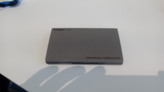
Model:  FC-1000 Financial Consultant

Company:  Casio

Years:  1988-early 1990s

Type:  Finance and Graphic

Batteries:  3 x CR-2025

Memory: 2,470 programming steps

Contrast wheel 


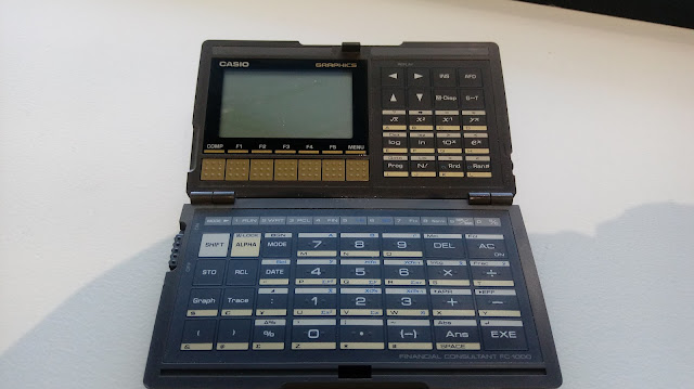
Like the Casio fx-7500G, the FC-1000 is a foldable calculator which is very small and light.  


Features


The main modes of the FC-1000 are come in two categories:  system modes and calculation modes.


System Modes


Run Mode (Mode 1):  This mode is for calculations and running programs.


Write Mode (Mode 2):  This mode is for writing programs, in one of 10 slots, Prog 0 to Prog 9.


Program Clear Mode (Mode 3):  Erase programs in this mode.  Clear all programs by pressing [ SHIFT ] [ DEL ] ( Mcl ).


Calculation Modes


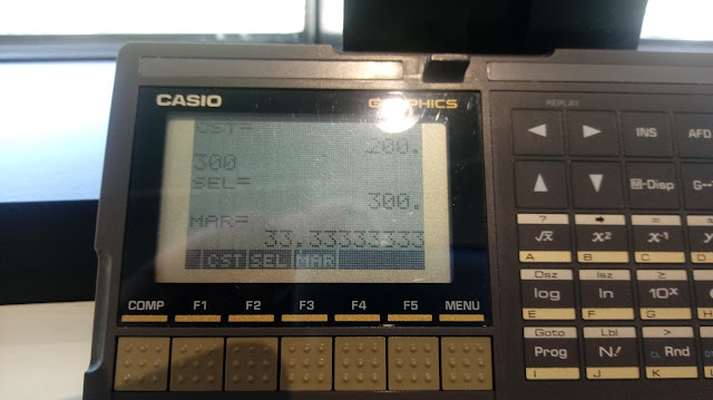
Financial Mode (Mode 4):  This mode is for financial calculations including time value of money (simple/compound/monthly C.I.), amortization, D.C.F. (discounted cash flows including NPV, IRR, NFV), bonds, depreciation, and cost/sell/margin.  The financial calculations are accessed by pressing the [ MENU ] key.   One of the great things of the FC-1000 is that it has a big screen to list variables and menu choices.  


Linear Regression Mode (Mode 5):  This mode fits bivariate data to the equation y = a + bx.  


SD Mode (Mode 6):  Single variable statistics


Mathematical Functions


The FC-1000 has a set of mathematical functions tailored to financial calculations:


*  powers and roots

*  logarithms

*  integer and fraction parts

*  factorials of positive integers

*  days between dates


How to figure out how to calculate days between dates:  


month_before [ DATE ] day_before [ DATE ] year_before [ DATE ] [ - ]

month_after [ DATE ] day_after [ DATE ] year_after [ DATE ]


If a two digit year is entered, it is implied that the year is 19##.  Thankfully four digits years are allowed, so this calculator can be used in the 21st century.   (Trivia:  I will be alive 16,436 days today using the 365 day mode).


The date separate is indicated by a forward slash.  


Programming 


The FC-1000 uses the Casio basic programming language.  The following commands available are:


Comparisons and the jump command:

[ test ] ⇒ [ do if true ] : or ◢  [ skip to here if false ]


Goto and label commands (Lbl 0-9)


Count jumps Isz (increment and skip on zero) and Dsz (decrement and skip on zero)


We can also store values in financial variables that are accessed through the menu system.  


As mentioned before, the space has a capacity of 2,470 steps over 10 program slots. 
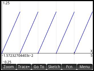

Graphing


The FC-1000 has graphing, but is limited to certain financial applications:  bonds, amortization, and depreciation.   Depending on what type of graph, pressing [ Trace ] will highlight the next period, and [ Shift ] [ Trace ] will rotate between different points of data.


For instance, in bonds, the [ Shift ] [ Trace ] combination rotates between price (PRC), coupon (CPN), and redemption value (RDV).


In amortization, the cycle is interest (INT), principal (PRN), and the nth payment (n).


In depreciation, the cycle is the year's depreciation (Depr) and year (n).  


Closing Thoughts


I love the form factor of the FC-1000 and how compact the calculator is.   However, the calculator is light weight and extra care is a must.  I wish the graphing module allowed us to graph functions and added statistical graphs.   


The FC-1000 can be difficult to collect, hence prices may be higher than a lot of vintage calculators.  


Until next time,


Eddie


All original content copyright, © 2011-2022.  Edward Shore.   Unauthorized use and/or unauthorized distribution for commercial purposes without express and written permission from the author is strictly prohibited.  This blog entry may be distributed for noncommercial purposes, provided that full credit is given to the author. 


Sunday, March 13, 2022

Casio fx-CG 50: Parametric Regression

Casio fx-CG 50:  Parametric Regression


Introduction


The program PARFIT2 attempts to pair data (x,y) using a pair of parametric equations [ x(t), y(t) ].   Each list of data will have its own curve.   


x(t), 1 ≤ t ≤ n

y(t), 1 ≤ t ≤ n

n = number of data points


Each point is assigned at t-value, which the program does automatically:

t = 1 refers to (x1, y1) → (t1, x1), (t1, y1)

t = 2 refers to (x2, y2) → (t2, x2), (t2, y2)

t = 3 refers to (x3, y3) → (t3, x3), (t3, y3)

and so on.


The program offers four regression types:


1.  Linear:  a + b*t

2.  Logarithm:  a + b*ln t

3.  Exponential:  a * b^t

4.  Power:  a * t^b


Variables used:


A = intercept for x(t)

B = slope for x(t)

R = correlation for x(t)


C = intercept for y(t)

D = slope for y(t)

S = correlation for y(t)


This allows for greater curve fitting control, which can accounts for different growth of the x data and y data, separately.


The program ends with a graph of the calculated parametric equation.  


Casio fx-CG 50 Program: PARTFIT


ClrText

Locate 1,1,"PARAMETRIC"

Locate 1,2,"FIT - 2022"

Locate 1,3,"EWS"

For 1→I To 750: Next

ParamType

ClrText

"X DATA"?→List 1

"Y DATA"?→List 2

Seq(x,x,1,Dim List 1, 1)→List 3


Menu "X=","A+BT",1,"A+Bln T",2,"A×B^T",3,"A×T^B",4

Lbl 1

LinearReg(a+bx) List 3, List 1

a→A: b→B: r→R

"A+BT"→Xt1

Goto 5

Lbl 2

LogReg List 3, List 1

a→A: b→B: r→R

"A+B×ln T"→Xt1

Goto 5

Lbl 3

ExpReg(a∙b^x) List 3, List 1

a→A: b→B: r→R

"A+B^T"→Xt1

Goto 5

Lbl 4

PowerReg List 3, List 1

a→A: b→B: r→R

"A+T^B"→Xt1

Goto 5

Lbl 5

"A, B, CORR=" ◢

[ [ A ] [ B ] [ R ] ] ◢


Menu "Y=","C+DT",A,"C+Dln T",B,"C×D^T",C,"C×T^D",D

Lbl A

LinearReg(a+bx) List 2, List 1

a→C: b→D: r→S

"C+DT"→Yt1

Goto E

Lbl B

LogReg List 2, List 1

a→C: b→D: r→S

"C+D×ln T"→Yt1

Goto E

Lbl C

ExpReg(a∙b^x) List 3, List 1

a→C: b→D: r→S

"C+D^T"→Yt1

Goto E

Lbl D

PowerReg List 3, List 1

a→C: b→D: r→S

"C+T^D"→Yt1

Goto E

Lbl E

"C, D, CORR=" ◢

[ [ C ] [ D ] [ S ] ] ◢


DrawGraph

ZoomAuto


Download the program here:  https://drive.google.com/file/d/1UVEHNZ7WILv3rSAgXy0_5kQ1lBPGEvKc/view?usp=sharing


Examples


Example 1:

(x,y):

(100.0, 10.0)

(101.3, 20.0)

(103.0, 31.7)

(104.3, 42.9)

(105.6, 54.2)

(107.0, 65.6)

(110.0, 77.0)


Fit x to linear and y to exponential.


Results:  

x(t) = 98.17142857 + 1.571428571*t,  corr = 0.9904886791

y(t) = 9.829695698 * 1.308085656^t, corr = 0.9639002639


Example 2:

(x,y):

(5.0, 0.41)

(2.9, 0.30)

(1.7, 0.20)

(0.9, 0.18)

(0.1, 0.12)


Fit x to logarithmic, y to power.


Results:  

x(t) = 5.002357022 - 3.010299732 * ln t, corr = -0.9997066364

y(t) = 0.4487684406* t^-0.7312889362,  corr = -0.9684707132


Eddie


All original content copyright, © 2011-2022.  Edward Shore.   Unauthorized use and/or unauthorized distribution for commercial purposes without express and written permission from the author is strictly prohibited.  This blog entry may be distributed for noncommercial purposes, provided that full credit is given to the author. 


Casio fx-CG50 and Swiss Micros DM32: HP 16C’s Bit Summation

  Casio fx-CG50 and Swiss Micros DM32: HP 16C’s Bit Summation The HP 16C’s #B Function The #B function is the HP 16C’s number of...