Sunday, January 31, 2021

HP 42S/DM42 and TI-85: True Bearing vs. Compass Bearing

 HP 42S/DM42 and TI-85:  True Bearing vs. Compass Bearing


Introduction 


The program converts angles between true bearing and compass bearing.


True Bearing:  0° to 360°, going clockwise from due north.  North is typically represented as the positive y direction.  True bearing is also known as azimuth.


Compass Bearing:  The grid is divided into four quadrants, each given one direction.  Measurements from each quadrant range from 0° to 90°.


Northeast (NE):  the angle is measured from true north (positive y axis), clockwise

Southeast (SE):  the angle is measured from true south (negative y axis), counterclockwise

Southwest (SW): the angle is measured from true south (negative y axis), clockwise

Northwest (NW): the angle is measured from true north (positive y axis), counterclockwise


HP 42S/DM42 Program:  CNVANG 


00 { 263-Byte Prgm }

01▸LBL "CNVANG"

02 DEG

03 "∡?"

04 PROMPT

05 STO 00

06 "∡ CONVERSION"

07 AVIEW

08 ">COMP"

09 KEY 1 GTO 01

10 "NE>"

11 KEY 2 GTO 06

12 "SE>"

13 KEY 3 GTO 03

14 "SW>"

15 KEY 4 GTO 04

16 "NW>"

17 KEY 5 GTO 05

18 MENU

19▸LBL 00

20 STOP

21 GTO 00

22▸LBL 01

23 CLA

24 360

25 MOD

26 ENTER

27 ENTER

28 90

29 MOD

30 STO 00

31 X<>Y

32 90

33 ÷

34 IP

35 STO 01

36 0

37 X=Y?

38 GTO 07

39 R↓

40 1

41 X=Y?

42 GTO 08

43 R↓

44 2

45 X=Y?

46 GTO 09

47 GTO 10

48▸LBL 07

49 RCL 00

50 ARCL ST X

51 32

52 XTOA

53 78

54 XTOA

55 69

56 XTOA

57 GTO 01

58▸LBL 08

59 90

60 RCL- 00

61 STO 00

62 ARCL ST X

63 32

64 XTOA

65 83

66 XTOA

67 69

68 XTOA

69 GTO 01

70▸LBL 09

71 RCL 00

72 ARCL ST X

73 32

74 XTOA

75 83

76 XTOA

77 87

78 XTOA

79 GTO 01

80▸LBL 10

81 90

82 RCL- 00

83 STO 00

84 ARCL ST X

85 32

86 XTOA

87 78

88 XTOA

89 87

90 XTOA

91 GTO 01

92▸LBL 01

93 BEEP

94 AVIEW

95 GTO 11

96▸LBL 03

97 180

98 X<>Y

99 -

100 GTO 06

101▸LBL 04

102 180

103 +

104 GTO 06

105▸LBL 05

106 360

107 X<>Y

108 -

109 GTO 06

110▸LBL 06

111 STO 00

112 BEEP

113 CLA

114 "TRUE="

115 ARCL ST X

116▸LBL 11

117 CLMENU

118 EXITALL

119 RTN

120 .END.


TI-85 Program: CONVANG


ClLCD

"2020-12-31 EWS"

Degree

Input "θ? ",A

Menu(1,">COMP",A1,2,"NE>",A2,3,"SE>",A3,4,"SW>,A4,5,"NW>",A5)

Lbl A1

mod(mod(A,360),90)→B

iPart(A/90)→C

If C==0

Then

Outpt(3,1,B)

Outpt(3,17,"° NE ")

End

If C==1

Then

90-B→B

Outpt(3,1,B)

Outpt(3,17,"° SE ")

End

If C==2

Then

Outpt(3,1,B)

Outpt(3,17,"° SW ")

End

If C==3

Then

90-B→B

Outpt(3,1,B)

Outpt(3,17,"° NW ")

End

Lbl A2

A→B

Goto A6

Lbl A3

180-A→B

Goto A6

Lbl A4

180+A→B

Goto A6

Lbl A5

360-A→B

Goto A6

Lbl A6

Outpt(3,1,"TRUE= ")

Outpt(3,7,B)

Stop


Examples


To True Bearing:

35 NE> returns 35

74 SE> returns 106

20 SW> returns 200

76 NW> returns 284


From True Bearing:

35 >COMP returns 35 NE

106 >COMP returns 74 SE

200 >COMP returns 20 SW

284 >COMP returns 76 NW


Coming up in February:  a review of the TI-36 XII calculator, more programs for an old favorite, the TI-85, and much more.


Here's to the Groundhog delivering great news on 2/2/2021,


Eddie


All original content copyright, © 2011-2021.  Edward Shore.   Unauthorized use and/or unauthorized distribution for commercial purposes without express and written permission from the author is strictly prohibited.  This blog entry may be distributed for noncommercial purposes, provided that full credit is given to the author. 


Saturday, January 30, 2021

TI-Nspire Python: Linear Regression

 TI-Nspire Python:  Linear Regression


Introduction


The following is a simple script to fit bivariate data using linear regression:


y = ax + b


a = slope

b = y-intercept


Download the document here:  https://drive.google.com/file/d/1trsa6oLdb0SG-1cHzog1stcbE6XY6BTv/view?usp=sharing


TI-Nspire Python Script:  linreg.py


# 2020-12-31 EWS

# linear regression 

from math import *


# enter and calculate data

xlist=[]

ylist=[]

n=int(input('n? '))

nb=0

sx=0

sx2=0

sy=0

sy2=0

sxy=0


for i in range(n):

  nb=nb+1

  print("Data Point "+str(nb))

  x=float(input('x? '))

  y=float(input('y? '))

  sx=sx+x

  sy=sy+y

  sx2=sx2+x**2

  sy2=sy2+y**2

  sxy=sxy+x*y

  xlist.append(x)

  ylist.append(y)


# slope

a=(sxy-sx*sy/nb)/(sx2-sx**2/nb)

# y-intercept

b=sy/nb-a*sx/nb

# correlation

r=(sxy-sx*sy/nb)/(sqrt(sx2-sx**2/nb)*sqrt(sy2-sy**2/nb))


# results

print("y = ax + b")

print("a= "+str(a))

print("b= "+str(b))

print("r= "+str(r))


The following script adds a plot of both the real and predicted data.


TI-Nspire Python Script:  linregplus.py


# 2020-12-31 EWS

# linear regression with plot

from math import *

import ti_plotlib as plt


# enter and calculate data

xlist=[]

ylist=[]

n=int(input('n? '))

nb=0

sx=0

sx2=0

sy=0

sy2=0

sxy=0


for i in range(n):

  nb=nb+1

  print("Data Point "+str(nb))

  x=float(input('x? '))

  y=float(input('y? '))

  sx=sx+x

  sy=sy+y

  sx2=sx2+x**2

  sy2=sy2+y**2

  sxy=sxy+x*y

  xlist.append(x)

  ylist.append(y)


# slope

a=(sxy-sx*sy/nb)/(sx2-sx**2/nb)

# y-intercept

b=sy/nb-a*sx/nb

# correlation

r=(sxy-sx*sy/nb)/(sqrt(sx2-sx**2/nb)*sqrt(sy2-sy**2/nb))


# results

print("y = ax + b")

print("a= "+str(a))

print("b= "+str(b))

print("r= "+str(r))


# predictive list

plist=[]

for i in range(n):

  p=a*xlist[i]+b

  plist.append(p)


# plot routine

# clear the screen

plt.cls()

# automatically fits the screen to fit the data

plt.auto_window(xlist,ylist)

# display the axes

# "on" plots axes and endpoints

# "axes" just plots the axes

plt.axes("on")


# select color - use RGB style

# denim blue, real data

plt.color(21,96,189)

plt.plot(xlist,ylist,".")

# orange, predictive data

plt.color(255,165,0)

plt.plot(xlist,plist,".")

# plot the graph

plt.show_plot()


Eddie


All original content copyright, © 2011-2021.  Edward Shore.   Unauthorized use and/or unauthorized distribution for commercial purposes without express and written permission from the author is strictly prohibited.  This blog entry may be distributed for noncommercial purposes, provided that full credit is given to the author. 


Sunday, January 24, 2021

HP 12C: Solving Two Actuarial Problems

 HP 12C: Solving Two Actuarial Problems


Solve for Interest and Number of Periods Given Present Value Annuity Factor and Future Value Annuity Factor


Given the following:


* Present Value Annuity Factor (PVAF)

* Future Value Annuity Factor (FVAF)


Solve for both:


*  the interest rate

*  the number of periods of the annuity


Keep in mind that present value and future value annuity factors are not the same of present value and future value, respectively.


Recall that:


PVAF = (1 - (1 + i)^-n) / i


FVAF = ((1 + i)^n - 1) / i


Note that:

FVAF = ( (1 + i)^n - 1 ) / i

FVAF = (1 + i)^n * (1 - (1+i)^-n) / i

FVAF= (1 + i)^n * PVAF


Then:

FVAF / PVAF = (1 + i)^n

ln (FVAF / PVAF) = ln (1 + i)^n

ln (FVAF / PVAF) = n * ln(1 + i)

ln (FVAF / PVAF) / ln(1 + i) = n


Also:

1 / FVAF + i 

= i / ((1 + i)^n - 1) + i

= i / ((1 + i)^n - 1) + (i * (1 + i)^n - 1)) / ((1+ i)^n - 1)

= (i + i * (1 + i)^n - i) / ((1 + i)^n - 1)

= (i * (1+i)^n) / ((1 + i)^n - 1)

= (1 + i)^n / (1 + i)^n * ( i / (1 - (1 + i)^-n)

= 1 * ( i / (1 - (1 + i)^-n)

= 1 / PVAF


Then:

1 / FVAF + i = 1 / PVAF

i = 1 / PVAF - 1 / FAVF


To summarize: 

i = 1 / PVAF - 1 / FAVF

n = ln (FVAF / PVAF) / ln(1 + i)


The following program solves for interest and number of payments. 


HP 12C (Classic) Program


Stack set up:

Y: PVAF

X:  FVAF


Step: Key: Code

01:  STO 1 :  44, 1

02:  x<>y :  34

03:  STO 2 :   44, 2

04:  1/x :   22

05:  x<>y :   34

06:  1/x :   22

07:  - :   30

08:  STO 3 :  44, 3

09:  ENTER :  36

10:  ENTER :  36

11:  1 :   1

12:  + :   40

13:   LN : 43, 23

14:  RCL 1 : 45, 1

15:  RCL 2 : 45, 2

16:  ÷  :  10

17:  LN :  43, 23

18:  x<>y : 34

19:  ÷  : 10

20:  STO 4 :  44, 4

21:  GTO 00 :  43, 33, 00


Example:


Input:

Y:  PVAF = 22.3965

X:  FVAF = 40.5681


Results:

Y:  i = 0.02   (2%)

X:  n = 30  (30 periods)


Present Value of an Annuity Due with an Effective Discount Rate


The problem determines the present value of an annuity due with an effective discount rate.  The effective discount rate is different from the interest rate (i).  Convert the effective discount rate to interest rate by:


i = d / (1 - d)   [i, d are in decimal form]


HP 12C (Classic) Program


Stack set up:

Clear TVM values

Store n:  [ n ]

Store payment: [ PMT ]

X:  discount rate (as a percentage.  Example: for 10%, enter 10)


Step: Key: Code

01:  BEG  : 43, 7

02:  ENTER  : 36

03:  CLx  :  35

04:  R↓   :  33

05:  1   :  1

06:  %  :  25

07:  1   :  1

08:  x<>y   :  34

09:  -  :  30

10:  LSTx  : 43, 36

11:  x<>y   :  34

12:  ÷  : 10

13:  1  :  1

14:  EEX  : 26

15:  2  :  2

16:  ×  :  20

17:  [ i ] :  12

18:  [ PV ]  :  13

19:  GTO 00  :  43,33,00


Example:


Input:

n = 36, PMT = -250.00

X:  d = 5%;  (5  [R/S])


Results:

X:  4211.10


Present Value:  $4,211.10


Source:


Finan, Marcel B.  A Basic Course in the Theory of Interest and Derivatives Markets:  A Preparation for the Actuarial Exam FM/2   Arkansas Tech University, 2017.  


Eddie


All original content copyright, © 2011-2021.  Edward Shore.   Unauthorized use and/or unauthorized distribution for commercial purposes without express and written permission from the author is strictly prohibited.  This blog entry may be distributed for noncommercial purposes, provided that full credit is given to the author. 


Saturday, January 23, 2021

Annuity Due in Terms of Ordinary Annuity

Annuity Due in Terms of Ordinary Annuity


Annuity:  Ordinary vs. Due


The distinction is determined when the first payment is made:


Ordinary Annuity:   the first payment is made at the end of the first period, with no payment made at the beginning (period 0) of the annuity. 


Annuity Due:  the first payment is made at the very beginning of the annuity, with no payment made at the end of the annuity.  


For today's exercise, assume all payments in annuity are all equal.  To simplify, I am going to set payments to 1 monetary unit (Dollars, Euros, Lira, Yen, etc).


Present Value


The present value of an annuity is today's value of the annuity, with future payments and cash flows are discounted back to today using the periodic interest rate.  On financial calculators, the present value is symbolized by the PV key.  


Let i be the interest rate of the annuity, in decimal format.  

Example, for 5% periodic rate, i=0.05.


Let v = 1/(1 + i).   


Present Value of an Ordinary Annuity


Given the payment of 1 monetary unit, an annuity of n periods, equally spaced out, and interest rate i, the present value of this ordinary annuity is the sum:


PVAF = v + v^2 + v^3 + ... + v^(n-1) + v^n = Σ(v^x for x=1 to n)


The above is known as the present value annuity factor, or PVAF.  


A closed formula for PVAF is:


PVAF = (1 - (1 + i)^-n) / i


Present Value of an Annuity Due


Likewise, the present value of the annuity due is the sum:


PVAFD = 1 + v + v^2 + v^3 + ... + v^(n-1) = Σ(v^x for x=0 to n-1)


A closed formula for PVAFD is:


PVAFD = (1 - (1 + i)^-n) / (1 - 1/(1 + i))


We can express PVAFD in terms of PVAF by:


PVAFD = 1 + v + v^2 + v^3 + ... + v^(n-1)

PVAFD + v^n = 1 + v + v^2 + v^3 + ... + v^(n-1) + v^n

PAVFD + v^n = 1 + PVAF

PAVFD = 1 + PVAF - v^n


PAVFD = 1 + (1 - (1 + i)^-n) / i - (1 + i)^-n


Example:  i = 0.04, n = 36


PAVFD = 1 + (1 - 1.04^-36) / 0.04 - 1.04^-36 ≈ 19.6646


This is the same as setting up TVM (time value of money) keys on most financial calculators or any calculator with a TVM solver as:

n = 36, I = 4, PMT = -1, FV = 0, (if needed, P/Y = 1),  BEGIN mode

Solve for PV:  19.6646...


Future Value


The future value of an annuity is the final value of the annuity, including the accumulated interest of payments and cash flows from the date the payment to the end of the annuity.  On financial calculators, the future value is symbolized by the FV key.  


Let w = 1 + i


Future Value of an Ordinary Annuity


Given the payment of 1 monetary unit, an annuity of n periods, equally spaced out, and interest rate i, the future value of this ordinary annuity is the sum:


FVAF = 1 + w + ... + w^(n-3) + w^(n-2) + w^(n-1) = Σ(w^x for x=0 to n-1)


The above is known as the future value annuity factor, or FVAR.  

A closed formula for FVAF is:


FVAF = ( (1 + i)^n - 1 ) / i


Future Value of an Annuity Due


Likewise, the future value of the annuity due is the sum:


FVAFD = w + ... + w^(n-3) + w^(n-2) + w^(n-1) + w^n = Σ(w^x for x=1 to n)


A closed formula for FVAFD is:


FVAFD = (1 + i) * ( (1 + i)^n - 1 ) / i 


We can express FVAFD in terms of FVAF by:


FAVFD = w + ... + w^(n-3) + w^(n-2) + w^(n-1) + w^n 

1 + FAVFD = 1 + w + ... + w^(n-3) + w^(n-2) + w^(n-1) + w^n 

1 + FAVFD = FAVD + w^n

FAVFD = FAVD + w^n - 1


FAVFD = ( (1 + i)^n - 1 ) / i + (1 + i)^n - 1


Example:  i = 0.04, n = 36


FAVFD = (1.04^36 - 1) / 0.04 + 1.04^36 - 1 ≈ 80.7022


Using the TVM keys or solver:

n = 36, I = 4, PMT = -1, PV = 0, (if needed, P/Y = 1),  BEGIN mode

Solve for FV:  80.7022...


On tomorrow's blog, January 24, I will cover two actuarial problems. 


Source:


Finan, Marcel B.  A Basic Course in the Theory of Interest and Derivatives Markets:  A Preparation for the Actuarial Exam FM/2   Arkansas Tech University, 2017.  


Eddie


All original content copyright, © 2011-2021.  Edward Shore.   Unauthorized use and/or unauthorized distribution for commercial purposes without express and written permission from the author is strictly prohibited.  This blog entry may be distributed for noncommercial purposes, provided that full credit is given to the author. 


Sunday, January 17, 2021

TI-Nspire: Templates to Plot Functions, Parametric Equations, and Sequences

 TI-Nspire:  Templates to Plot Functions, Parametric Equations, and Sequences


Introduction


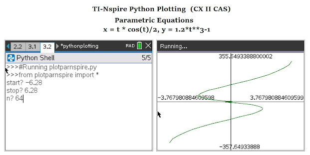
The following are sample templates to plot functions in the form of y=f(x), parametric equations (x(t), y(t)), and one-level deep recurrence relations.


I used a while loop instead of a for loop because I tend to always use for loops, and working with integer objects can be quite difficult for non-Python experts like me.  


The equations will be defined inside the script instead of having the user enter the script.  .   I am using the TI-NSpire CX II software 5.2.0771.  I have programmed this with the TI-Nspire CX CAS software, but it should work on the non-CAS version.  


As far as entering numbers at the input prompt, I have to enter approximations for π (which is approximately 3.1415926535).  


The list.append(value) or list.append(list) adds the elements to the end of the list and the list is automatically saved.  


The graphic commands uses a TI-specific module ti_plotlib.  I have a lot of pleasure working with this module, with commands for clearing the graphic screen, automatically sizing the window, plotting the axes, with or without the numeric numeric endpoints, and set a color with RGB codes (any color you want).  


You can download the file here:  https://drive.google.com/file/d/1k_3lTVK5KK1ACXrVxemSWz_g-l8Nn62A/view?usp=sharing


The text of the scripts are presented below.


Plotting Functions -   TI-Nspire CX II (CAS) Script:  plotfxnspire.py


from math import *

import ti_plotlib as plt


# EWS 2020-12-28


# define function here

def f(x):

  y=1/(x**2+1)

  return y


# main routine

xa=float(input('start? '))

xb=float(input('stop? '))

n=float(input('n? '))

xc=(xb-xa)/n


# build

xp=xa

yp=f(xp)

xlist=[xp]

ylist=[yp]


while xp<xb:

  xp=xp+xc

  yp=f(xp)

  xlist.append(xp)

  ylist.append(yp)


# plot routine

# clear the screen

plt.cls()

# automatically fits the screen to fit the data

plt.auto_window(xlist,ylist)

# display the axes

# "on" plots axes and endpoints

# "axes" just plots the axes

plt.axes("on")


# select color - use RGB style

# denim blue

plt.color(21,96,189)


# plot the graph

plt.plot(xlist,ylist,".")

plt.show_plot()


Plotting Parametric Equations -   TI-Nspire CX II (CAS) Script:  plotparnspire.py


from math import *

import ti_plotlib as plt


# EWS 2020-12-28


# define parametric here

def x(t):

  x=t*cos(t)/2

  return x

def y(t):

  y=1.2*t**3-1

  return y


# main routine

ta=float(input('start? '))

tb=float(input('stop? '))

n=float(input('n? '))

tc=(tb-ta)/n


# build

tp=ta

xp=x(tp)

yp=y(tp)

xlist=[xp]

ylist=[yp]


while tp<tb:

  tp=tp+tc

  xp=x(tp)

  yp=y(tp)

  xlist.append(xp)

  ylist.append(yp)


# plot routine

# clear the screen

plt.cls()

# automatically fits the screen to fit the data

plt.auto_window(xlist,ylist)

# display the axes

# "on" plots axes and endpoints

# "axes" just plots the axes

plt.axes("on")


# select color - use RGB style

# mid green

plt.color(0,128,0)


# plot the graph

plt.plot(xlist,ylist,".")

plt.show_plot()


Plotting a Recurrence Relation-   TI-Nspire CX II (CAS) Script:  plotseqnspire.py


Use u for u_n-1.  You should also be able to include n without problems.  


from math import *

import ti_plotlib as plt


# EWS 2020-12-28


# define sequence here, u for u(n-1)

def w(u):

  w=cos(u)+1

  return w


# main routine

ui=float(input('initial? '))

n=float(input('n? '))


# build

xlist=[0]

ylist=[ui]

k=0


while k<n:

  k=k+1

  f=w(k)

  xp=k

  yp=f

  xlist.append(xp)

  ylist.append(yp)


# plot routine

# clear the screen

plt.cls()

# automatically fits the screen to fit the data

plt.auto_window(xlist,ylist)

# display the axes

# "on" plots axes and endpoints

# "axes" just plots the axes

plt.axes("on")


# select color - use RGB style

# orange

plt.color(255,127,39)


# plot the graph

plt.plot(xlist,ylist,".")

plt.show_plot()


Eddie


All original content copyright, © 2011-2021.  Edward Shore.   Unauthorized use and/or unauthorized distribution for commercial purposes without express and written permission from the author is strictly prohibited.  This blog entry may be distributed for noncommercial purposes, provided that full credit is given to the author. 

Saturday, January 16, 2021

Numworks: Templates to Plot Functions, Parametric Equations, and Sequences

 Numworks:  Templates to Plot Functions, Parametric Equations, and Sequences


Introduction


The following are sample templates to plot functions in the form of y=f(x), parametric equations (x(t), y(t)), and one-level deep recurrence relations.


I used a while loop instead of a for loop because I tend to always use for loops, and working with integer objects can be quite difficult for non-Python experts like me.  


The equations will be defined inside the script instead of having the user enter the script.  If anyone knows how to use input to enter functions, please let me know.   I am using Numworks software version 14.4.  


As far as entering numbers at the input prompt, I have to enter approximations for π (which is approximately 3.1415926535).  The plot screen is made to fit the y-minimum and y-maximum values within the window.


The list.append(value) or list.append(list) adds the elements to the end of the list and the list is automatically saved.  


The named colors, which is required in matplolib.pyplot, available are:  'black', 'blue', 'brown', 'green', 'grey', 'orange', 'pink', 'purple', 'red', 'white', and 'yellow'.


Plotting Functions -   Numworks Script:  plotfunction.py


from math import *

from matplotlib.pyplot import *

# EWS 2020-12-26


# define function here

def f(x):

  y=1/(x**2+1)

  return y


# main routine

xa=float(input('start? '))

xb=float(input('stop? '))

n=float(input('n? '))

xc=(xb-xa)/n


# build

xp=xa

yp=f(xp)

xlist=[xp]

ylist=[yp]


while xp<xb:

  xp=xp+xc

  yp=f(xp)

  xlist.append(xp)

  ylist.append(yp)


# plot routine


# set axes

ya=min(ylist)

yb=max(ylist)

axis((xa,xb,ya,yb))

axis(True)

grid(True)


# select color, type color

ch="blue"


# plot points

plot(xlist,ylist,color=ch)

show()


Plotting Parametric Equations -   Numworks Script:  plotparametric.py


from math import *

from matplotlib.pyplot import *

# EWS 2020-12-26


# define parametric here

def x(t):

  x=t**2-3*t+1

  return x

def y(t):

  y=abs(2*sin(t))

  return y


# main routine

ta=float(input('start? '))

tb=float(input('stop? '))

n=float(input('n? '))

tc=(tb-ta)/n


# build

tp=ta

xp=x(tp)

yp=y(tp)

xlist=[xp]

ylist=[yp]


while tp<tb:

  tp=tp+tc

  xp=x(tp)

  yp=y(tp)

  xlist.append(xp)

  ylist.append(yp)


# plot routine


# set axes

xa=min(xlist)

xb=max(xlist)

ya=min(ylist)

yb=max(ylist)

axis((xa,xb,ya,yb))

axis(True)


# select color, type color

ch="red"


# plot points

plot(xlist,ylist,color=ch)

show()


Plotting a Recurrence Relation-   Numworks Script:  plotsequence.py


Use u for u_n-1.  You should also be able to include n without problems.  


from math import *

from matplotlib.pyplot import *

# EWS 2020-12-26


# define parametric here

# u: u(n-1)

def w(u):

  f=sqrt(3*u+1)

  return f


# main routine

ui=float(input('initial? '))

n=float(input('n? '))


# build

xlist=[0]

ylist=[ui]

k=0


while k<n:

  k=k+1

  f=w(k)

  xp=k

  yp=f

  xlist.append(xp)

  ylist.append(yp)


# plot routine


# set axes

ya=min(ylist)

yb=max(ylist)

axis((0,n,ya,yb))

axis(True)


# select color, type color

ch="green"


# plot points

plot(xlist,ylist,color=ch)

show()


On tomorrow's blog, January 17, 2021, I am going to present these scripts for the TI-Nspire CX II.   I used the CX CAS software, but this should work on the CX (non-CAS) calculator and software as well.  

Eddie


All original content copyright, © 2011-2021.  Edward Shore.   Unauthorized use and/or unauthorized distribution for commercial purposes without express and written permission from the author is strictly prohibited.  This blog entry may be distributed for noncommercial purposes, provided that full credit is given to the author. 


Sunday, January 10, 2021

Casio fx-9750GIII: Trigonometric Integral Graphs, including The Euler Spiral

 Casio fx-9750GIII:  Trigonometric Integral Graphs, including The Euler Spiral


Introduction


The program ESGRAPH plots the parametric equations containing integrals:


x(t) = ∫(cos f(x) dx, x = 0 to t)

y(t) = ∫(sin f(x) dx, x = 0 to t)


The program uses f(x) = a*x^p


When p = 2, the curve is a Euler Spiral (see source).


Casio fx-9750GIII Program: ESGRAPH


' 2020-12-22 EWS

Rad

' L1, X L2, Y

"F = A×X^P"

"FACTOR"?→A

"P=2, EULER SPIRAL"

"POWER"?→P

∫(A×cos(X^P),0,-2π)→X

∫(A×sin(X^P),0,-2π)→Y

{X}→List 1

{Y}→List 2

Menu "π÷R?","8",A,"16",B,"32",C

Lbl A: 8 → R: Goto 0

Lbl B: 16 → R: Goto 0

Lbl C: 32 → R : Goto 0

Lbl 0

For -2π+π÷R→T To 2π Step π÷R

∫(A×cos(X^P),0,-2π)→X

∫(A×sin(X^P),0,-2π)→Y

Augment(List 1, {X})→List 1

Augment(List 2, {Y})→List 2

(T+2π)÷(4π)×100→G

RndFix(G,0)→G

Locate 1,7,"PROGRESS:    %"

Locate 11,7,G

Next

S-Gph1 DrawOn, xyLine, List 1, List 2, 1, Dot

DrawStat


Notes:


*  There are four spaces between PROGRESS: and %.  This progress meter is to inform the user of the program's completion. 


*  The characters % and ', percent sign and apostrophe respectively, are found on the program editing default menu (TOP, BTM, SRC, MENU, A ←→a, CHAR), by pressing [F6] (CHAR), [F2] (SYBL)


*  Everything that follows an apostrophe is a comment and can be left out.


*  The range of -2π to 2π is used. 


*  The lower the precision, the faster the graph is made but accuracy of the graph is sacrificed.  In a lot of cases, patience is required. 


*  P is a positive integer.  


Examples


Example 1:  Euler Spiral:  A = 1/2, P = 2, precision 32


Example 2:  A = 1, P  = 3, precision 32


Example 3:  A = 2, P = 1, precision 16


Source:


Havil, Julian.  Curves for the Mathematical Curious: An Anthology of the Unpredictable, Historical, Beautiful, and Romantic  Princeton Universal Press. Princeton and Oxford. Princeton, NJ 2019 ISBN 978-0-691-18005-2


Eddie


All original content copyright, © 2011-2021.  Edward Shore.   Unauthorized use and/or unauthorized distribution for commercial purposes without express and written permission from the author is strictly prohibited.  This blog entry may be distributed for noncommercial purposes, provided that full credit is given to the author. 


Saturday, January 9, 2021

TI 84 Plus: Plotting Circular Arcs with Just Two Points

 TI 84 Plus: Plotting Circular Arcs with Just Two Points


Introduction


Knowing two points (x0, y0) and (x1, y1), we can draw a circular arc between two points.  We are going to assume that the points form the diameter of the circle.  Therefore, either point forms the radius along with the line's midpoint.   The midpoint between the points, labeled (A,B) is:


A = (x0 + x1) / 2, B = (y0 + y1) / 2


With the radius:


R = √((A - x0)^2 + (B - y0)^2) = √((x1 - A)^2 + (y1 - B)^2)


Set the parametric equations as:


x = R * (cos(t) + A / R)

y = R * (sin(t) + B / R)


With t being the range of required angle measure (θ), we have to determine the start and end points for the range of values for t.  Since (A, B) may not be the origin, we must take it into account the midpoint in determining the angle points:


t0 = atan((B - y0) / (A - x0)) mod 2*π

t1 = atan((y1 - B) / (x1 - A)) mod 2*π


The program ARC2PTS for the TI-84 Plus makes use the complex number functions abs and angle to determine radius and the angles, respectively.


TI-84 Plus Program: ARC2PTS


"2020-12-20 EWS"

Radian

a+bi

Param

FnOff 

Input "X0? ",J

Input "Y0? ",K

Input "X1? ",L

Input "Y1? ",M

(J+L)/2→A

(K+M)/2→B

angle((A-J)+i(B-K))→C

If C<0:C+2π→C

angle((A-L)+i(B-M))→D

If D<0:D+2π→D

abs((A-J)+i(B-K))→R

"R(cos(T)+A/R)"→X₁T

"R(sin(T)+B/R)"→Y₁T

Menu("DIRECTION","TOP",1,"BOTTOM",2)

Lbl 1

min(C,D)→Tmin

max(C,D)→Tmax

Goto 3

Lbl 2

max(C,D)→Tmin

min(C,D)+2π→Tmax

Goto 3

Lbl 3

π/64→Tstep

ZoomFit

ZSquare


Examples


Example 1


Points:  (1,3) and (5,9), top part of the circle


Example 2


Points:  (-5, -8) and (-1, -7), bottom part of the circle


Eddie


All original content copyright, © 2011-2021.  Edward Shore.   Unauthorized use and/or unauthorized distribution for commercial purposes without express and written permission from the author is strictly prohibited.  This blog entry may be distributed for noncommercial purposes, provided that full credit is given to the author. 


Sunday, January 3, 2021

Swiss Micros DM42 and HP71B: Present Value of a Growing Annuity

Swiss Micros DM42 and HP71B: Present Value of a Growing Annuity


Introduction


Today we are going to calculate the present value of a growing annuity.  Unlike most annuities where the payment is constant, in a growing annuity, the payment increases each period.  For this particular blog, we are working with annuities that payments increase by a growth percent (g%) each period.  The annuity has an different interest rate (r%) in which payments are discounted.  


Since the payments are not constant, the time value of money (TVM) keys on a financial calculator are not going to be used.  If your calculator has the the net present value (NPV) function, this can assist you in these calculations.

I am going to use a different approach.


Derivation


Variables:


P = base payment (the first payment)

g = growth rate per period 

r = interest rate per period

n = number of periods 

PV = present value


Ordinary Growing Annuity


In an ordinary growing annuity, the first payment will be received after one period (typically a year or a month) has passed.  Discounting all the payments to calculate present value:


PV 

=  P/(1+r) + P * (1+g)/(1+r)^2 + P * (1+g)^2/(1+r)^3 + ... + P * (1+g)^(n-1)/(1+r)^n

=  P/(1+r) * [ 1 + (1+g)/(1+r) + (1+g)^2/(1+r)^2 + ... + (1+g)^(n-1)/(1+r)^(n-1)


Let w = (1+g)/(1+r), then:


PV

= P/(1+r) * [ 1 + w + w^2 + ... + w^(n-1) ]


The result is a geometric series.  In a general geometric series:


a + a*r + a*r^2 + ... + a*r^(n-1) = Σ(a*r^k, k=0 to n-1) = a * (1 - r^n)/(1 - r)


Then:


PV

= P/(1+r) * [ 1 + w + w^2 + ... + w^(n-1) ]

= P/(1+r) * Σ(w^k, k=0 to n-1) 

= P/(1+r) * (1 - w^n)/(1 - w)


Alternatively, change w back to (1+g)/(1+r):


PV

= P/(1+r) * (1 - (1+g)^n/(1+r)^n) / (1 - (1+g)/(1+r))

= [ P/(1+r) * (1 - (1+g)^n/(1+r)^n) ] / [ 1 - (1+g)/(1+r) ]

= [ P/(1+r) * P/(1+r) * (1+g)^n/(1+r)^n ] / [ 1 - (1+g)/(1+r) ]


The article from finaceformulas.net (see source) suggests multiplying by (1+r) / (1+r):


= [ P/(1+r) - P/(1+r) * (1+g)^n/(1+r)^n ] / [ 1 - (1+g)/(1+r) ] * (1 + r) / (1 + r)

= [ P - P * (1+g)^n/(1+r)^n ] / [ 1 + r - (1 + g) ]

= [ P - P * (1+g)^n/(1+r)^n ] / [ r - g ]

= P / (r - g) * (1 - (1+g)^n/(1+r)^n )


Growing Annuity Due


On an annuity due, the first payment takes place immediately.  The present value is calculated as:


PV 

=  P +  P * (1+ g)/(1+r) + P * (1+g)^2/(1+r)^2 + P * (1+g)^3/(1+r)^3 + ... + P * (1+g)^n/(1+r)^n

=  P * [ 1 + (1+ g)/(1+r) + (1+g)^2/(1+r)^2 + (1+g)^3/(1+r)^3 + ... + (1+g)^n/(1+r)^n ]


Let w = (1+g)/(1+r), then:


PV 

= P * [1 + w + w^2 + w^3 + ... + w^n ]


We have another geometric progression:


PV 

= P  * (1 - w^(n+1))/(1 - w)


Summary:


Present Value of a Growing Annuity - Ordinary


PV = P/(1+r) * (1 - w^n)/(1 - w)


Present Value of a Growing Annuity - Due


PV = P  * (1 - w^(n+1))/(1 - w)


HP 42S/DM42 Program:  PVGROW


Both PVGROW and PVGDUE use only one register, R01.


00  {79-Byte Prgm}

01  LBL "PVGROW"

02  "BASE PMT?"

03  PROMPT

04  "INTEREST?"

05  PROMPT

06  1

07  X<>Y

08  %

09  +

10  STO 01

11  ÷

12  1

13  "GROWTH?"

14  PROMPT

15  %

16  +

17  RCL÷ 01

18  STO 01

19  "N?"

20  PROMPT

21  Y↑X

22  1

23  X<>Y

24  -

25  1

26  RCL- 01

27  ÷

28  ×

29  "PV="

30  ARCL ST X

31  AVIEW

32  END


HP 42S/DM42 Program:  PVGDUE


00  {79-Byte Prgm}

01  LBL "PVGDUE"

02  "BASE PMT?"

03  PROMPT

04  "INTEREST?"

05  PROMPT

06  1

07  X<>Y

08  %

09  +

10  1

11  "GROWTH?"

12  PROMPT

13  %

14  +

15  ÷

16  1/X

17  STO 01

18  "N?"

19  PROMPT

20  1

21  +

22  Y↑X

23  1

24  X<>Y

25  -

26  1

27  RCL- 01

28  ÷

29  ×

30  "PV="

31  ARCL ST X

32  AVIEW

33  END


HP 71B Program: PVGROW


Note:  This is for both ordinary and growing annuities due.


100  DESTROY P,G,R,W,A,C

105  INPUT "PAYMENT? "; P

110  INPUT "INTEREST? "; R

115  R=.01*R

120  INPUT "GROWTH? "; G

125  G=.01*G

130  W=(1+G)/(1+R)

135  INPUT "N? "; N

140  INPUT "DUE?(Y=1,N=0) ";C

145  IF C=1 THEN 200

150  IF C=0 THEN 300 ELSE 140 


200  A=P*(1-W^(N+1))/(1-W) @ ! DUE

205  GOTO 400


300  A=P*(1-W^N)/((1+R)*(1-W)) @ ! ORD

305 GOTO 400


400 PRINT "PV ="; A


Examples:


Base Payment:  P = 20.00

Interest Rate:  r = 4%

Growth Rate:  g = 5%

n = 5


Ordinary Growing Annuity


Result:  PV = 98.02


Timeline of Payments:

Period 0:  0.00

Period 1:  20.00

Period 2:  21.00

Period 3:  22.05

Period 4:  23.15

Period 5:  24.31


Growing Annuity Due


Result:  PV = 122.92


Period 0:  20.00

Period 1:  21.00

Period 2:  22.05

Period 3:  23.15

Period 4:  24.31

Period 5:  25.53


Source:


"Present Value of a Growing Annuity" financeformulas.net  https://financeformulas.net/Present_Value_of_Growing_Annuity.html   Retrieved December 13, 2020.  


Eddie


All original content copyright, © 2011-2021.  Edward Shore.   Unauthorized use and/or unauthorized distribution for commercial purposes without express and written permission from the author is strictly prohibited.  This blog entry may be distributed for noncommercial purposes, provided that full credit is given to the author. 


Saturday, January 2, 2021

Retro Review: Radio Shack EC-4018

 Retro Review:   Radio Shack EC-4018


HAPPY NEW YEAR!


Quick Facts:


Company:  Radio Shack

Model:  EC-4018

Equivalent of:  Casio fx-470

Type:  Scientific 

Years:  Late 1980's

Display:  10 digits

Batteries:  Solar

Memory Registers: 1


Keyboard


The keyboard of the EC-4018 is a folding landscape.    The top half has the screen and 18 gray keys (scientific) to the right side, and two solar panel strips to the left.  The bottom half has 15 large black keys (arithmetic).  I really like the large keys on this calculator.  The keys are really easy to press and operated, and they also have a nice feel to them.  


Features


*  Trigonometric functions, logarithms, powers, rots

*  Convert to and from degrees-minutes-seconds

*  Four base conversions:  binary, decimal, octal, hexadecimal

*  Boolean Algebra: AND, OR, XOR, NEG

*  Fractions, combinations, permutations, reciprocal, factorials of integers


Physical Constants


INV 1:  Speed of Light in a Vacuum: c =  299792458 m/s

INV 2:  Planck's Constant:  h = 6.626176 * 10^-34 J s 

INV 3:  Universal Gravitational Constant:  G = 6.672 * 10^-11 N m^2/kg^2

INV 4:  Elementary Charge:  e = 1.6021892 * 10^-19 C

INV 5:  Electron Rest Mass:  me = 9.109534 * 10^-31 kg

INV 6:  Atomic Mass Unit:  u = 1.6605655 * 10^-27 kg

INV 7:  Avogadro's Constant:  Na = 6.022045 * 10^23/mol

INV 8:  Boltzmann Constant:  k = 1.308662 * 10^-23 J/K

INV 9:  Molar Volume of Ideal Gas:  Vm = 0.02241383 m^3/mol


According to the Casio fx-650 manual, these values are based on 1978 Japan Industrial Standards.  


The nice thing is that the units are stated next to the symbol.  


Verdict 


I am really like the keyboard and the contrast of the font colors.  The bright orange and gold really stand out against the black keyboard.   The screen's digits are really nice and big.  As I mentioned before, the keys have a nice feel.  


If you like a folding scientific calculator, you are going to have to search for a vintage calculator.  The good thing about Radio Shack is that their calculators tend to be less expensive than Casio.  


Sources:


"Electronic Calculators"  epocalc.net  Last Updated April 25, 2013.  http://www.epocalc.net/pages/mes_calcs_03.htm   Retrieved December 12, 2020.


Casio fx-650 Operation Manual


Eddie


All original content copyright, © 2011-2021.  Edward Shore.   Unauthorized use and/or unauthorized distribution for commercial purposes without express and written permission from the author is strictly prohibited.  This blog entry may be distributed for noncommercial purposes, provided that full credit is given to the author. 


Spotlight: Sharp EL-5200

  Spotlight: Sharp EL-5200 As we come on the 13 th (April 16) anniversary of this blog, I want to thank you. Blogging about mathematic...