Solving Simple Arcsine and Arccosine Equations

 Solving Simple Arcsine and Arccosine Equations

Angle Measure

This document will focus on angle measurement in degrees. For radians and grads, please use the appropriate measurement.

90° = π/2 rad = 100 grad

180° = π rad = 200 grad

Simple Arcsine Equations

The calculator arcsine function gives: Domain: -1 ≤ x ≤ 1, Range: -90° ≤ Θ ≤ 90°

Note that for any angle x: sin(180° - x) = sin(x), sin(x) = sin(x ± 360°*z) (z is an integer)

Given n, solve for Θ:

n = sin(Θ) = sin(180° - Θ)

Base Solution 1:

n = sin(Θ)

⇒ Θ = arcsin(n)

Base Solution 2:

n = sin(180° - Θ)

arcsin(n) = 180° - Θ

⇒ Θ = 180° - arcsin(n)

Example:

0.67 = sin(Θ)

Base Solution 1: Θ = arcsin(0.67) ≈ 42.0670648025°

Base Solution 2: Θ = 180° - arcsin(0.67) ≈ 137.932935198°

Given n and α, solve for Θ:

n = sin(α + Θ)

Base Solution 1:

n = sin(α + Θ)

arcsin(n) = α + Θ

⇒ Θ = arcsin(n) – α

Base Solution 2:

n = sin(180° - (α + Θ))

n = sin(180° - α – Θ)

arcsin(n) = 180° - α – Θ

⇒ Θ = 180° - α – arcsin(n)

Example:

0.7757 = sin(Θ + 76°)

Base Solution 1: Θ = arcsin(0.7757) – 76° ≈ -25.1314549842°

Base Solution 2: Θ = 180° - 76° - arcsin(0.7757) = 104° - arcsin(0.7757) ≈ 53.131459842°

To get all the possible angles, add and subtract multiples of 360°.

Solving Simple Arccosine Equations

The calculator arccosine function gives: Domain: -1 ≤ x ≤ 1, Range: -90° ≤ Θ ≤ 90°

Note that for any angle x: cos(180° - x) = -cos(x), cos(x) = cos(x ± 360°*z) (z is an integer)

Given n, solve for Θ:

n = cos(Θ), n = cos(-Θ)

Base Solution 1:

n = cos(Θ)

⇒ Θ = arccos(n)

Base Solution 2:

n = cos(-Θ)

⇒ Θ = -arccos(n)

Example:

0.58 = cos(Θ)

Base Solution 1: Θ = arccos(0.58) ≈ 54.54945736°

Base Solution 2: Θ = -arccos(0.58) ≈ -54.54945736°

Given n and α, solve for Θ:

n = cos(α + Θ)

Base Solution 1:

n = cos(α + Θ)

arccos(n) = α + Θ

⇒ Θ = arccos(n) – α

Base Solution 2:

n = cos(-(α + Θ))

n = cos(-α – Θ)

arccos(n) = -α – Θ

-arccos(n) = α + Θ

⇒ Θ = -arccos(n) – α

Example:

0.6 = cos(35° + Θ)

Base Solution 1: Θ = arccos(0.6) – 35° ≈ 18.13012035°

Base Solution 2: Θ = -arccos(0.6) – 35° ≈ -88.13010235°

To get all the possible angles, add and subtract multiples of 360°.

I hope you find this useful and helpful,

Eddie

All original content copyright, © 2011-2026. Edward Shore. Unauthorized use and/or unauthorized distribution for commercial purposes without express and written permission from the author is strictly prohibited. This blog entry may be distributed for noncommercial purposes, provided that full credit is given to the author.

HP 12C: Quickly Approximating Arc Tangent

HP 12C: Quickly Approximating Arc Tangent

The HP 12C does not have trigonometric functions. Various sources list on how such functions are be approximated with varying degrees of accuracy. Today’s blog will feature a quick approximation, using only a 14 step function for the arc tangent (inverse tangent) function.

Formula Used in Approximation

(see Source)

arctan(x) ≈ x ÷ (1 + 0.28125 * x²) = x ÷ (1 + 9 * x² ÷ 32)

Best for -1 ≤ x ≤ 1

Maximum absolute error of 0.0049 radians, approximately 0.28°. The error gets worse outside these ranges. The program rounds the result to 2 decimal places. The angle is returned in radians.

HP 12C Program: Arc-tangent Approximations

FIX 2	01	42, 2	Program start
ENTER	02	36
ENTER	03	36
×	04	20
9	05	9
×	06	20
3	07	3
2	08	2
÷	09	10
1	10	1
+	11	40
÷	12	10
RND	13	42, 14	Round result to 2 decimal places
GTO 00	14	43, 33, 00	Program end

Examples

x = 0.1. Result: 0.10

x = 0.3. Result: 0.29

x = 0.5. Result: 0.47

Source

Sreeraman Rajan, Sichun Wang, Rober Inkol, and Alain Joyal. “Efficient Approximations for the Arctangent Function” IEEE Signal Processing Magazine. May 2006.

Eddie

All original content copyright, © 2011-2026. Edward Shore. Unauthorized use and/or unauthorized distribution for commercial purposes without express and written permission from the author is strictly prohibited. This blog entry may be distributed for noncommercial purposes, provided that full credit is given to the author.

Trigonometric Calculus when Angles are in Degrees

Trigonometric Calculus when Angles are in Degrees

Today’s blog is a quickie.

The preferred angle measure in calculus is the radian. However, a lot of applications, including geometry, astronomy, engineering, and construction, use degrees.

An approach is to convert everything to radians before proceeding. Another approach is to remember that x radians = x° * π / 180, and use the conversion factor.

Derivatives

d/dx sin( x° )

Now all calculus calculations must have radians.

d/dx sin( x * π / 180)

= π / 180 * cos (x * π / 180)

= π / 180 * cos(x°)

Similarly – remember the angle considered is in DEGREES:

d/dx sin(x°) = π / 180 * cos(x°)	d/dx csc(x°) = - π / 180 * csc(x°) * cot(x°)
d/dx cos(x°) = - π / 180 * sin(x°)	d/dx sec(x°) = π / 180 * tan(x°) * sec(x°)
d/dx tan(x°) = π / 180 * sec(x°)^2	d/dx cot(x°) = -π / 180 * csc(x°)

Integration

Now let’s try integration.

∫( sin(x°) dx)

= ∫( sin(x * π / 180)) dx

= 180 / π * ∫(π / 180 * sin(x * π / 180)) dx

= 180 / π * -cos(x * π / 180) + C

= -180 / π * cos(x°) + C

Similarly:

∫ sin(x°) dx = -180 / π * cos(x°) + C

∫ cos(x°) dx = 180 / π * sin(x°) + C

∫ tan(x°) dx = -180 / π * ln(cos(x°)) + C

Use caution when using calculators. A lot of calculators when using calculus in degree mode get it correct but its’ always good to verify.

Eddie

All original content copyright, © 2011-2025. Edward Shore. Unauthorized use and/or unauthorized distribution for commercial purposes without express and written permission from the author is strictly prohibited. This blog entry may be distributed for noncommercial purposes, provided that full credit is given to the author.

The author does not use AI engines and never will.

TI-30Xa Algorithms: RLC Series Circuit

TI-30Xa Algorithms: RLC Series Circuit

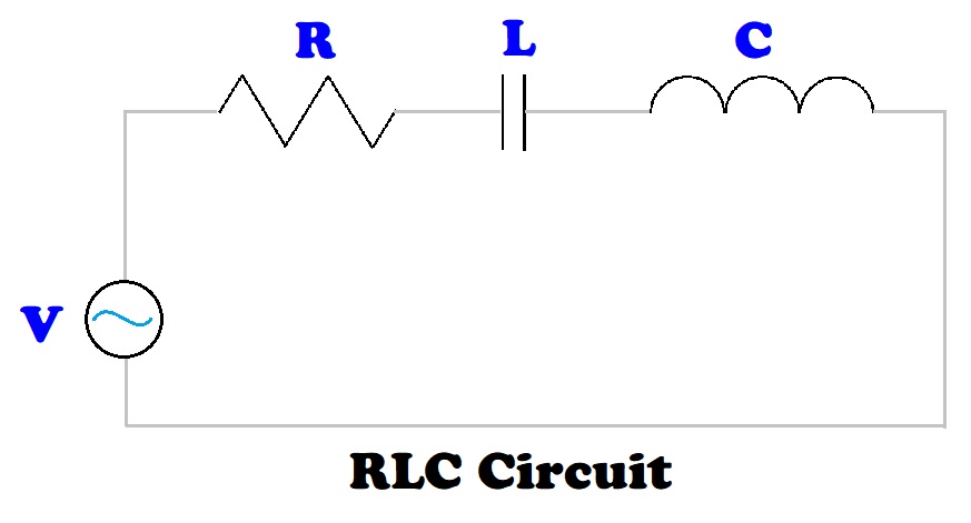
The task is to calculate the total impedance and phase angle for an RLC circuit in a series. An RLC circuit contains a resistor ( R ), an inductor ( L ), and a capacitor ( C ) , all powered by a voltage supply. The resistor, inductor, and capacitor are all in a single path.

The three elements are measured in the following units:

Resistor ( R ): Ohms ( Ω )

Inductor ( L ): Henry ( H )

Capacitor ( C ): Farads ( F )

The impedance for the RLC circuit is calculated by:

Z = √( R^2 + ( (2 * π * f * L) - 1 / (2 * π * f * C) )^2 )

The phase angle is calculated by:

θ = arctan( ( (2 * π * f * L) - 1 / (2 * π * f * C) ) / R )

where: f = frequency in Hertz (Hz)

We can use the rectangular to polar conversion function (R>P) to calculate both the impedance and phase angle.

x = R

y = (2 * π * f * L) - 1 / (2 * π * f * C)

If we have an RL circuit, with no capacitor, then C = 0.

If we have an RC circuit, with no inductor, then L = 0.

If we have an LC circuit, with no resistor, then R = 0.

TI-30Xa Algorithm – RLC Circuit

Step 1: Store resistance in Memory 1.

R [ STO ] 1

Step 2: Calculate angular frequency, ω = 2 * π * f, store in memory 3.

2 [ × ] [ π ] [ × ] f [ = ] [ STO ] 3

Step 3: Calculate (2 * π * f * L) - 1 / (2 * π * f * C)

[ RCL ] 3 [ × ] L [ - ] [ ( ] [ RCL ] 3 [ × ] C [ ) ] [ 1/x ] [ = ] [ STO ] 2

If we have an RL circuit, Steps 2 and 3 can be shortened to:

2 [ × ] [ π ] [ × ] f [ × ] L [ = ] [ STO ] 2

If we have an RC circuit, Steps 2 and 3 can be shortened to:

[ ( ] 2 [ × ] [ π ] [ × ] f [ × ] C [ ) ] [ 1/x ] [ +/- ] [ = ] [ STO ] 2

Step 4: Calculate Impedance and Phase Angle:

[ RCL ] 1 [ 2^nd ] [ π ] (x<>y) [ RCL ] 2 [ 2^nd ] [ - ] (R>P)

What is shown: (r) Impedance

Press [ 2^nd ] [ π ] (x<>y) for phase angle (θ)

Examples

Example 1: RLC Series Circuit

R = 50 Ω

L = 3.8 H

C = 0.7 F

f = 40 Hz

Step 1: Store resistance in Memory 1.

50 [ STO ] 1

Step 2: Calculate angular frequency, ω = 2 * π * f, store in memory 3.

2 [ × ] [ π ] [ × ] 40 [ = ] [ STO ] 3 (251.3274123)

Step 3: Calculate (2 * π * f * L) - 1 / (2 * π * f * C)

[ RCL ] 3 [ × ] 3.8 [ - ] [ ( ] [ RCL ] 3 [ × ] 0.0007 [ ) ] [ 1/x ] [ = ] [ STO ] 2

(949.36000616)

Step 4: Calculate Impedance and Phase Angle:

[ RCL ] 1 [ 2^nd ] [ π ] (x<>y) [ RCL ] 2 [ 2^nd ] [ - ] (R>P)

Impedance: 950.6758262

Phase Angle: 86.9851854°

Example 2: RLC Series Circuit

R = 450 Ω

L = 1.15 H

C = 3.5 μF = 3.5 * 10^-6 F

f = 60 Hz

Step 1: Store resistance in Memory 1.

450 [ STO ] 1

Step 2: Calculate angular frequency, ω = 2 * π * f, store in memory 3.

2 [ × ] [ π ] [ × ] 60 [ = ] [ STO ] 3 (376.9911184)

Step 3: Calculate (2 * π * f * L) - 1 / (2 * π * f * C)

[ RCL ] 3 [ × ] 1.15 [ - ] [ ( ] [ RCL ] 3 [ × ] 3.5 [ EE ] 6 [ +/- ] [ ) ] [ 1/x ] [ = ] [ STO ] 2

(-324.3408952)

Step 4: Calculate Impedance and Phase Angle:

[ RCL ] 1 [ 2^nd ] [ π ] (x<>y) [ RCL ] 2 [ 2^nd ] [ - ] (R>P)

Impedance: 554.7044405

Phase Angle: -35.78246242°

Source

“Impedance and Complex Impedance” Electronics Tutorials. AspenCore, Inc. 2024. Retrieved October 7, 2024. https://www.electronics-tutorials.ws/accircuits/impedance.html

This wraps up the TI-30Xa Algorithm Series. Next up will be a series on the Casio fx-991CW.

I want to wish you all a Happy New Year and a prosperous, sane, and happy 2025! Be safe, everyone, it’s a very crazy world we live in.

Eddie

All original content copyright, © 2011-2024. Edward Shore. Unauthorized use and/or unauthorized distribution for commercial purposes without express and written permission from the author is strictly prohibited. This blog entry may be distributed for noncommercial purposes, provided that full credit is given to the author.

Swiss Micros DM32: Spherical Triangle ft. Law of Cosines

Swiss Micros DM32: Spherical Triangle ft. Law of Cosines

Introduction

The state file spheretri.d32 is about solving triangles on the spherical space.

The programs solve spherical triangles in two common problems: SSS (side-side-side, really arc lengths) and SAS (side-angle-side). All the inputs are in decimal degrees.

Also calculated are the surface area and perimeter, both in radians. The radius is assumed to be 1.

Surface Area = ( A° + B° + C° ) * π / 180 – π = A + B + C – π

Perimeter = ( X° + Y° + Z°) * π / 180 = X + Y + Z

The sum of the angles (A, B, C) must be greater than 180° (π radians). Due to this requirement, in solving for angles and sides, the Law of Cosines will be used in each instance. The Law of Sines is only advised to check ratios.

Equation listing

Law of Sines – can be used as a check on triangles:

SIN(A)÷SIN(X)=SIN(B)÷SIN(Y)

Law of Cosines – two equations:

COS(Z)=COS(X)×COS(Y)+SIN(X)×SIN(Y)×COS(C)

COS(C)=-COS(A)×COS(B)+SIN(A)×SIN(B)×COS(Z)

Here the variables are general place holders.

Program Listing

Labels:

Label H: help program

Label I: Initialization routine. Sets the angles mode to degrees and clears the variables.

Label C: Starts the solve spherical triangle routine: given the three arc lengths X, Y, and Z.

Label Z: Starts the solve spherical triangle routine: given the arc lengths X and Y and and the angle between the arcs, angle C

Label F: Routine to solve for angles A and B, perimeter, and area

General Instructions

1. To start a new problem, execute program I.

2. To solve a spherical triangle given the sides (arc lengths), execute program C. (SSS)

3. To solve a spherical triangle given two sides and the internal angle, execute program Z. (SAS)

This program also solves for the surface area, assuming a radius of 1, and perimeter of the triangle.

Program Code

H01 LBL H

H02 SF 10

H03 EQN: A N G L E _ A _ B _ C

H04 EQN: S I D E S _ X _ Y _ Z

H05 EQN: X E Q _ C _ S S S

H06 EQN: X E Q _ Z _ S A S

H07 EQN: E Q N S _ A R E _ S I N E

H08 EQN: A N D _ C O S I N E _ L A W S

H09 CF 10

H10 RTN

I01 LBL I

I02 DEG

I03 CLVARS

I04 CLx

I05 RTN

C01 LBL C

C02 INPUT X

C03 INPUT Y

C04 INPUT Z

C05 RCL Z

C06 COS

C07 RCL X

C08 COS

C09 RCL Y

C10 COS

C11 ×

C12 -

C13 RCL X

C14 SIN

C15 RCL Y

C16 SIN

C17 ×

C18 ÷

C19 ACOS

C20 STO C

C21 VIEW C

C22 XEQ F

C23 RTN

Z01 LBL Z

Z02 INPUT X

Z03 INPUT Y

Z04 INPUT C

Z05 RCL X

Z06 COS

Z07 RCL Y

Z08 COS

Z09 ×

Z10 RCL X

Z11 SIN

Z12 RCL Y

Z13 SIN

Z14 ×

Z15 RCL C

Z16 COS

Z17 ×

Z18 +

Z19 ACOS

Z20 STO Z

Z21 VIEW Z

Z22 XEQ F

Z23 RTN

F01 LBL F

F02 RCL X

F03 COS

F04 RCL Z

F05 COS

F06 RCL Y

F07 COS

F08 ×

F09 -

F10 RCL Z

F11 SIN

F12 RCL Y

F13 SIN

F14 ×

F15 ÷

F16 ACOS

F17 STO A

F18 RCL Y

F19 COS

F20 RCL X

F21 COS

F22 RCL Z

F23 COS

F24 ×

F25 -

F26 RCL X

F27 SIN

F28 RCL Z

F29 SIN

F30 ×

F31 ÷

F32 ACOS

F33 STO B

F34 RCL A

F35 RCL+ B

F36 RCL+ C

F37 →RAD

F38 π

F39 -

F40 STO R

F41 RCL X

F42 RCL+ Y

F43 RCL+ Z

F44 →RAD

F45 STO P

F46 VIEW A

F47 VIEW B

F48 VIEW R

F49 VIEW P

F50 RTN

You can download the DM32 state file here:

https://drive.google.com/file/d/1qX-y2G5sCOmm4ktmZbnGoPI3uzrx6IfF/view?usp=sharing

Examples  (FIX 5)

SSS Problem (LBL C)

X = 18.66°

Y = 20.49°

Z = 19.95°

Results:

C = 62.04726°

A = 55.92702°

B = 64.98954°

R = 0.05173 radians (surface area)

P = 1.03149 radians (perimeter)

SAS Problem (LBL Z)

X = 17.00 °

Y = 23.32°

C = 64.55°

Results:

Z = 21.88733°

A = 45.08768°

B = 73.51096 °

R = 0.05495 radians (surface area)

P = 1.08572 radians (perimeter)

Sources

Wikipedia. “Spherical Triangle” Updated April 9, 2024. Retrieved April 11, 2024.

https://en.wikipedia.org/wiki/Spherical_trigonometry#:~:text=Spherical%20trigonometry%20is%20the%20branch,sphere%2C%20geodesics%20are%20great%20circles.

Gray, Glen. “Spherical Trigonometry – An Introduction and Basic Theorems” Video. February 12, 2023. Retrieved April 11, 2024. https://www.youtube.com/watch?v=McWv9bcvMYg

Note: The blog will be posted on Saturdays only on June and July 2024.

Eddie

All original content copyright, © 2011-2024. Edward Shore. Unauthorized use and/or unauthorized distribution for commercial purposes without express and written permission from the author is strictly prohibited. This blog entry may be distributed for noncommercial purposes, provided that full credit is given to the author.