Today's session is about starting other apps in a program and using colors.
Defining equations in the Program Editor and Home
The equation must be a string and be stored to the appropriate designated variable.
F# is for functions of X. (Function app).
R# is for polar functions of θ. (Polar app).
U# is for sequences of N, N-1, N-2. (Sequence app).
X# and Y# for parametric equations of T. (Parametric App)
V# for open statements and equations in the Advanced Graphing App, which The independent variables are X and Y.
# is a digit 0-9.
Defining equations this way leaves them uncheck. If you want them plotted or accessed in Num View, you will need to check them.
Example:
F1:="2*X^3" stores the function f(x) = 2*x^3 in Function 1.
R5:="A*SIN(θ)" stores the polar function r(θ) = A*sin(θ) in Polar Function 5, with A being what value stored in it.
STARTAPP
STARTAPP(application name in quotes);
Starts the named App. The calculator points the screen to the default view (Plot, Symb, Num).
Access: Cmds, 4. App Functions, 2. STARTAPP
CHECK and UNCHECK
Checks and unchecks specific equation or function (0-9) in the current app. For example, if you are in the Function app, CHECK(1) activates F. As you should expect, UNCHECK(1) turns F1 off.
What does CHECK and UNCHECK affect?
1. Whether a function is plotted in Plot view.
2. Whether a function is analyzed in Num view.
Access for CHECK: Cmds, 4. App Functions, 1. CHECK
Access for UNCHECK: Cmds, 4. App Functions, 4. UNCHECK
STARTVIEW
Instructs the HP Prime to go to a certain view. It has two arguments, the view number and a redraw number.
Common view numbers include (not all inclusive):
-2 = Modes screen
-1 = Home
0 = Symbolic (Symb)
1 = Plot
2 = Numeric (Num)
3 = Symbolic Setup
4 = Plot Setup
5 = Numeric Setup
6 = App Information
7 = The Views Key
8 = first special view
9 = second special view
Etc..
The redraw number is either 0 or non-zero. 0 does not redraw the screen, anything else does. I recommend the latter.
Syntax: STARTVIEW(view number, redraw number)
Access: Cmds, 4. App Functions, 3. STARTVIEW
RGB
Returns an integer code pertaining to a color's RGB code. This is super useful for drawing and text writing.
Syntax: RGB(red, green, blue, alpha)
Red: Intensity of Red, 0-255
Green: Intensity of Green, 0-255
Blue: Intensity of Blue, 0-255
Alpha: (optional) Opacity (up to 128).
RGB codes:
Blue: RGB(0,0,255)
Violet: RGB(143,255,0)
Dark Green: RGB(0,128,0)
Orange: RGB(255,127,0)
Yellow: RGB(0,255,255)
Red: RGB(255,0,0)
White: RGB(255,255,255)
Black: RGB(0,0,0)
Gray: RGB(129,128,128)
Brown: RGB(150,75,0)
Light Blue: RGB(173,216,330)
For other colors, RGB can be found on various sites on the Internet, including Wikipedia.
Access: Cmds, 2. Drawing, 5. RGB
Tip: Change a color of a graph
Use the syntax
F#(COLOR):=RGB(red,blue,green,[alpha]);
F stands for the designated function type (F for function, R for polar, etc)
# is the digit 0-9.
Example:
F8(COLOR):=RGB(0,0,255)
makes the function F8 plot in blue.
This is a lot, but this is doable. Let's see all these commands and tips in action and create some magic.
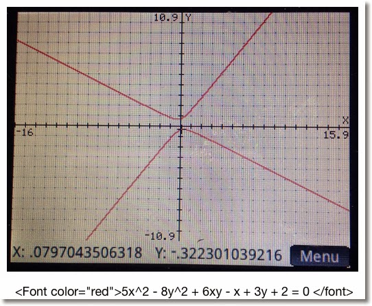
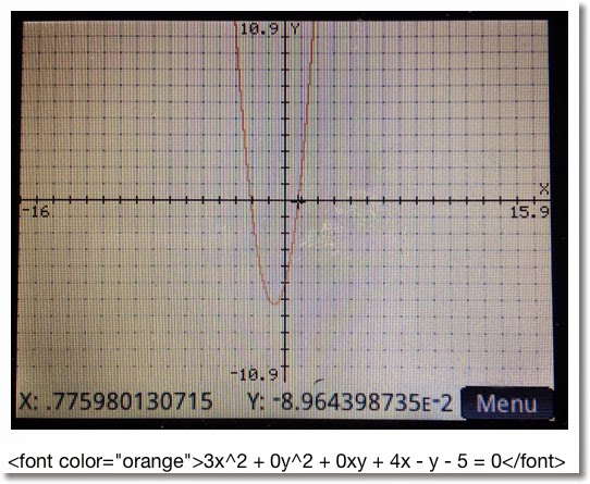
Conic Drawing for HP Prime
Draws the conic section for the general equation
Ax^2 + By^2 + Cxy + Dx + Ey + F = 0
You can choose the color how the conic section is plotted, from red, blue, orange, and green. (Game show enthusiasts take note of the order of the colors I listed... ;) ).
EXPORT CONIC()
BEGIN
LOCAL cr, cg, cb, I;
INPUT({A,B,C,D,E,F},
"Ax^2+By^2+Cxy+Dx+Ey+F", { }, { },
{0,0,0,0,0,0});
// Colors
CHOOSE(I, "Choose a Color",
"Red","Blue","Orange","Green");
cr:={255,0,255,0};
cg:={0,0,127,255};
cb:={0,255,0,0};
STARTAPP("Advanced Graphing");
V1:="A*X^2+B*Y^2+C*X*Y+D*X+E*Y+F=0";
V1(COLOR):=RGB(cr(I),cg(I),cb(I));
CHECK(1);
// Plot View
STARTVIEW(1,1);
END;
Below are some examples. Remember the form:
Ax^2 + By^2 + Cxy + Dx + Ey + F = 0


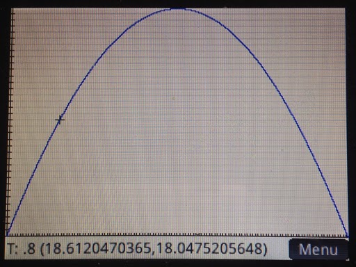
Projectile Motion for HP Prime
This program calculates range and height of a projectile, and plots its path. The program sets the mode into Degrees (HAngle=1) and the calculator to the Parametric app.
Equations:
x = V * cos θ * t
y = V * sin θ * t - .5 * g * t^2
Where
V = initial velocity
θ = initial degree of flight
g = Earth gravitation constant (9.80665 m/s^2, ≈32.17404 ft/s^2)
Air resistance is not factored, so we are dealing with ideal conditions. How much the projectile represents reality varies, where factors include the object being projected, the temperate and pressure of the air, and the weather.
EXPORT PROJ13()
BEGIN
LOCAL M, str;
// V, G, θ are global
// Degrees
HAngle:=1;
CHOOSE(M, "Units", "SI", "US");
IF M==1 THEN
str:="m";
G:=9.80665;
ELSE
str:="ft";
G:=32.17404;
END;
INPUT({V, θ}, "Data",
{"V:","θ:"},
{"Initial Velocity in "+str+"/s",
"Initial Angle in Degrees"});
X1:="V*COS(θ)*T";
Y1:="V*SIN(θ)*T-.5*G*T^2";
STARTAPP("Parametric");
CHECK(1);
// Adjust Window
Xmin:=0
// Range
Xmax:=V^2/G*SIN(2*θ);
Ymin:=0
// Height
Ymax:=(V^2*SIN(θ)^2)/(2*G);
MSGBOX("Range: "+Xmax+" "+str+", "
+", Height: "+Ymax+" "+str);
// Plot View
STARTVIEW(1,1);
END;
Below are screen shots from an example with V = 35.25 m/s and θ = 48.7°.

This concludes this session of the tutorials. Shortly I will have Part 6 up, which has to do routines.
I am catch-up mode, still. But then again I always feel like there is too much to do and too little time. LOL
See you soon!
Eddie
This blog is property of Edward Shore. 2013