Showing posts with label random numbers. Show all posts

Sunday, March 15, 2026

TI-84 Plus CE Python: Traceable Plots in Python

TI-84 Plus CE Python: Traceable Plots in Python


These two scripts are an easy way on how to create plots that are traceable. A traceable plot allows the user to trace along a scatter plot or functional plot by using the right and left arrow keys, just like if you made a plot in a graphing calculators’ graph mode.


The two scripts presented are:


TIRNDPLT: makes a scatter plot of ten random points between 0 and 1. The x axis is the plot marker while the y axis is the random point.

TIFXPLT: makes a plot of a single function y(x). Radians mode as assumed and the plot is made of 50 points. You specify the minimum and maximum values of x. Radians mode is assumed and the math module has imported, allowing for scientific functions. A caveat is to plot a function where it is defined for all of the domain given. For instance, for sqrt(x), no negative values should be included in the domain [xmin, xmax].


The two scripts can be downloaded here:

https://drive.google.com/file/d/1D3oB7Vrt9cd1e-wXrEkhZbr8VJ_7V4qB/view?usp=sharing


However I am going to list the code because there are things to be pointed out.


TIRNDPLT


Code:

# TI-84+: Traceable Plot

# Edward Shore 2026-02-20
# tirndplt.py

# Plot ten random elements

# import modules
from math import *
from random import *
from ti_system import *
# plot module is imported differently
import ti_plotlib as plt


# build a random list
x=[i for i in range(1,11)]
y=[round(random(),4) for i in range(1,11)]

# set up the key
# left (2) and right (1) is the trace, enter to exit (5)
k=0

# set the pointer
p=0

# constant elements
# clear the screen
plt.cls()
# set window to allow room for text
plt.window(0,11,-0.5,1.5)
plt.axes("axes")

# plot gray grid
plt.color(192,192,192)
plt.grid(1,0.1)

# main loop, faster?, redraw only replaceable elements
while k!=5:
  # scatter plot, filled dot default
  plt.color(0,0,0)
  plt.scatter(x,y)
  # text at line 1
  plt.text_at(1,"<-, ->, press enter to exit","left",1)
  # string at line 12
  s="x = {0:.0f}, y = {1:.4f}".format(x[p],y[p])
  plt.text_at(12,s,"left",1)
  # plot pointer with cross, blue
  plt.color(0,0,255)
  plt.plot(x[p],y[p],"x")
  # get key
  k=wait_key()
  # left and right keys
  if k==2:
    # clear
    plt.color(255,255,255)
    plt.plot(x[p],y[p],"x")
    # replace
    plt.color(0,0,0)
    plt.plot(x[p],y[p])
    p=(p-1)%10
  elif k==1:
    plt.color(255,255,255)
    plt.plot(x[p],y[p],"x")
    plt.color(0,0,0)
    plt.plot(x[p],y[p])
    p=(p+1)%10

# show draw at the end
plt.text_at(1,"DONE","left",1)
plt.show_plot()


Notes:


1. Modules used: math, random, ti_system, and ti_plotlib. The calling of math and random modules allow the user to include math and random functions. The ti_system has the command wait_key(), which calls for the user to press a key, and returns a specific code value when a key is pressed. The module ti_plotlib is for the specific graphics commands.

2. The y minimum and maximum values for the plot have a padding of 2 to allow room for the top and bottom lines which will contain information. The top line will give instructions for the keys: ← to trace left, → to trace right, and pressing the [ enter ] exits the program.

3. The script has plots in two sections. Outside the loop are elements that will stay permanent: the window, the axis, and the scatter plot. Inside the loop will be the pointer because it changes.

4. Every time an arrow key is processed, the pointer first must be “erased” off the previous position, then move to the next. The pointer is in blue. The variable p is used for the pointer and will take the value between 0 and 9.

5. In Python, the percent symbol is used as a modulus function. So, the expression (p-1)%10 means (p – 1) mod 10. Similarly, (p+1)%10 means (p + 1) mod 10. This is what keeps p in the range of [0, 9]. p is an integer.

6. The use of the format is required to make reading the coordinates readable.

7. Any script using ti_plotlib must have a plt.show_plot() command, at least at the end. It’s primary purpose is to show the final picture and freeze the screen in graphics mode.


TIFXPLT.py


Code:

# TI-84+: Traceable Plot
# Edward Shore 2026-02-22
# tifxplt.py


# Plot a traceable function

# import modules
from math import *
from random import *
from ti_system import *
# plot module is imported differently
import ti_plotlib as plt

# build f(x)
fx=input("y(x)? ")
xmin=eval(input("xmin? "))
xmax=eval(input("xmax? "))
chgx=(xmax-xmin)/50

xl=[]
yl=[]

x=xmin
while x<=xmax:
  y=eval(fx)
  xl.append(x)
  yl.append(y)
  x+=chgx

ymin=min(yl)-2
ymax=max(yl)+2

# set up the key
# left (2) and right (1) is the trace, enter to exit (5)
k=0

# set the pointer
p=0

# constant elements
# clear the screen
plt.cls()
# set window to allow room for text
plt.window(xmin,xmax,ymin,ymax)
plt.color(16,16,16)
plt.axes("on")

plt.color(0,0,0)
plt.plot(xl,yl,".")

# main loop, faster?, redraw only replaceable elements
while k!=5:
  # scatter plot, filled dot default
  # text at line 1
  plt.text_at(1,"<-, ->, press enter to exit","left",1)
  # string at line 12
  s="x = {0:.1f}, y = {1:.4f}".format(xl[p],yl[p])
  plt.text_at(12,s,"left",1)
  # plot pointer with cross, blue
  plt.color(0,0,255)
  plt.plot(xl[p],yl[p],"x")
  # get key
  k=wait_key()
  # left and right keys
  if k==2:
    # clear
    plt.color(255,255,255)
    plt.plot(xl[p],yl[p],"x")
    # replace
    plt.color(0,0,0)
    plt.plot(xl[p],yl[p])
    p=(p-1)%50
  elif k==1:
    plt.color(255,255,255)
    plt.plot(xl[p],yl[p],"x")
    plt.color(0,0,0)
    plt.plot(xl[p],yl[p])
    p=(p+1)%50

# show draw at the end
plt.text_at(1,"DONE","left",1)
plt.show_plot()


Notes:

1. Modules used: math, random, ti_system, and ti_plotlib. The calling of math and random modules allow the user to include math and random functions. The ti_system has the command wait_key(), which calls for the user to press a key, and returns a specific code value when a key is pressed. The module ti_plotlib is for the specific graphics commands.

2. The y minimum and maximum values for the plot have a padding of 2 to allow room for the top and bottom lines which will contain information. The top line will give instructions for the keys: ← to trace left, → to trace right, and pressing the [ enter ] exits the program.

3. The script has plots in two sections. Outside the loop are elements that will stay permanent: the window, the axis, and the plot of the function. Inside the loop will be the pointer because it changes.

4. Every time an arrow key is processed, the pointer first must be “erased” off the previous position, then move to the next. The pointer is in blue. The variable p is used for the pointer and will take the value between 0 and 49.

5. In Python, the percent symbol is used as a modulus function. So, the expression (p-1)%50 means (p – 1) mod 50. Similarly, (p+1)%50 means (p + 1) mod 50. This is what keeps p in the range of [0, 49]. p is an integer.

6. The use of the format is required to make reading the coordinates readable.

7. Any script using ti_plotlib must have a plt.show_plot() command, at least at the end. It’s primary purpose is to show the final picture and freeze the screen in graphics mode.


I hope you enjoy these programs as I did making them,


Eddie


All original content copyright, © 2011-2026. Edward Shore. Unauthorized use and/or unauthorized distribution for commercial purposes without express and written permission from the author is strictly prohibited. This blog entry may be distributed for noncommercial purposes, provided that full credit is given to the author.

Saturday, January 4, 2025

Casio fx-CG 50: Pseudorandom Number Generator (PRNG) Stat Plot

Casio fx-CG 50: Pseudorandom Number Generator (PRNG) Stat Plot


Introduction


This program is an inspiration from a HHC 2024 talk given by Kuba Tatarkiewicz. Tatarkiewicz’s talk is about testing RNG (random number generators). You can see it here: https://www.youtube.com/watch?v=vSDfqCK-ENk


Premise of RANDGRPH: Generate a recursive sequence


r_n = frac( (A * r_n-1 + B) ^ C)


The program builds two lists and develops a scatter plot. I have the program set up to plot 60 points, but we can up to 999 points. The list starts with the initial point (0, seed). The program asks you whether to have the calculator provide the seed or you provide a seed (between 0 and 1).


Casio fx-CG 50 Code: RANDGRPH (252 bytes)


“RAN # GRAPH”

“(A×R+B)^C” ◢

“A”? → A

“B”? → B

“C”? → C

Menu “SEED?”, “RANDOM”, 1, “YOUR OWN”, 2

Lbl 1

Ran# → R

Goto 0

Lbl 2

“0≤R<1, SEED”? → R

Lbl 0

{0} → List 1

{R} → List 2

For 1 → I To 75

Augment(List 1, {R}) → List 1

Frac((A×R+B)^C) → R

Augment(List 2,{R}) → List 2

Next

S-Gph1 DrawOn, Scatter, List 1, List 2, 1, Dot, ColorLinkOff, Black, AxesOn

DrawStat


Examples


Example 1: r_n = frac(991 * r_n-1)


r_n = frac(991 * r_n-1)


Example 2: r_n = frac( (0.3 * r_n-1 + 1)^2 )


r_n = frac( (0.3 * r_n-1 + 1)^2 )


Example 3: r_n = frac( (r_n-1 + π)^5 )


r_n = frac( (r_n-1 + π)^5 )


Enjoy! Happy New Year, be safe, sane, strong, and take care. Forever grateful,


Eddie


All original content copyright, © 2011-2025. Edward Shore. Unauthorized use and/or unauthorized distribution for commercial purposes without express and written permission from the author is strictly prohibited. This blog entry may be distributed for noncommercial purposes, provided that full credit is given to the author.

Saturday, January 13, 2024

TI-30Xa Algorithms: Probability

TI-30Xa Algorithms:  Probability


Introduction


Even when a calculator isn't (technically) programmable, algorithms can be applied to scientific and financial calculations.


The calculations take numerical arguments that are stored in the TI-30Xa's three memory slots:  M1, M2, and M3.  Store amounts into the memory registers by the [ STO ] key.  


Careful:  For the solar versions of the TI-30Xa, do not press the [ON/AC] button as doing so clears the memory registers.


The registers used:


M1 = n 

M2 = k 

M3 = p 


Repeated Combinations


nHk = (n + k -1)Ck = (n + k - 1)! ÷ (k! × (n - 1)!)


Registers:


M1:  n = number of objects

M2:  k = number of objects chosen in the population


nHk = number of combinations of picking k from n objects, assuming repeats are allowed


Algorithm:


[ ( ] [ RCL ] 1 [ + ] [ RCL ] 2 [ - ] 1 [ ) ] [ 2nd ] (nCr) [ RCL ] 2 [ = ]


Example:


M1: n = 50

M2: k = 5


Result:  3,162,510


Binomial Probability Distribution


Prob(k) = nCk × p^k × (1 - p)^(n - k) = n! ÷ (k! × (n - k)!) × p^k × (1 - p)^(n - k) 


Registers:


M1:  n = number of trials

M2:  k = number of successes

M3:  p = probability of success (in decimal; i.e. enter 0.30 for 30%)


Prob =  probability of k successes out of n trials with a success probability p


Algorithm:  


[ RCL ] 1 [ 2nd ] (nCr) [ RCL ] 2 [ × ] [ RCL ] 3 [ y^x ] [ RCL ] 2 [ × ] [ ( ] 1 [ - ] [ RCL ] 3  [ ) ] [ y^x ] [ ( ] [ RCL ] 1 [ - ] [ RCL ] 2 [ ) ] [ = ] 


Example:


M1: n = 50

M2: k = 5

M3: p = 0.8


Result:  2.442763967 × 10^-26


Geometric Probability Distribution


Prob(k) = (1 - p)^(k - 1) × p


Registers:


M2:  k = number of failures before the first success

M3:  p = probability of success (in decimal) 


Prob = probability of a event taking k trials before the first success


Algorithm:


[ ( ] 1 [ - ] [ RCL ] 3 [ ) ] [ y^x ] [ ( ] [ RCL ] 2 [ - ] 1 [ ) ] [ × ] [ RCL ] 3 [ = ]


Example:


M2: k = 5

M3: p = 0.8


Result:  0.00128


A Simple Pseudorandom Number Generator


The TI-30Xa does not have a random number function.  To generate random numbers, a pseudorandom number generator algorithm must be used in the form of:


x_n+1 = f(x_n)


where x_0 is the initial value, known as the seed value.  


A simple pseudorandom  number generator to generate numbers between 0 and 1 is:


x_n+1 = frac(997 × x_n + π)


Algorithm:


With x_n in display:

[ × ] 997 [ + ] [ π ] [ = ] 

[ - ] the integer part of the number in the display [ = ]


Result:  x_n+1.   


There is no fraction part or integer part functions are not available on the TI-30Xa.  


Example:   


Starting seed:   0.7896   


[ × ] 997 [ + ] 

[ π ] [ = ]        Display:  799.3457927

[ - ] 799 [ = ]  Display:  0.345792654


[ × ] 997 [ + ] 

[ π ] [ = ]        Display:  347.8968683

[ - ] 347 [ = ]  Display:  0.896868283


[ × ] 997 [ + ] 

[ π ] [ = ]        Display:  897.3192706

[ - ] 897 [ = ]  Display:  0.319270625


[ × ] 997 [ + ] 

[ π ] [ = ]        Display:  321.4544059

[ - ] 321 [ = ]  Display:  0.454405908


and so on...


The random numbers with the starting seed 0.7896 are:

0.345792654

0.896868283

0.319270625

0.454405908


Take as many decimal points as you wish.  


If you enjoy this post, I will consider making a series using the TI-30Xa calculator (and similar simple scientific calculators).  Until next time,


Eddie 


All original content copyright, © 2011-2024.  Edward Shore.   Unauthorized use and/or unauthorized distribution for commercial purposes without express and written permission from the author is strictly prohibited.  This blog entry may be distributed for noncommercial purposes, provided that full credit is given to the author. 


Sunday, December 24, 2023

TI-73 (Explorer): Percents and Random Fractions

TI-73 (Explorer):  Percents and Random Fractions


TI-73 Program:  PERCENT


TAX+:  Appropriately add a percent to a number.   Application:  Sales Tax


TAX-:   Appropriately subtract a percent from a number.  Application:  Discount


% CHANGE:  Percent change from the old number to new number.  Additional application:  Percent Markup (OLD = cost, NEW = selling price)


%TOT:  Finds the percentage portion of a total number


% MARGIN:  Given an item's cost and selling price, calculate the item's percent margin.  


Code:

(spaces added for clarity)


"EWS 2023-12-02"     // (comment)


Lbl 0

Menu("PERCENT","TAX+",1,"TAX-",2,

"% CHANGE",3,"%TOT",4,"% MARGIN",5,

"EXIT",E)


Lbl 1

Prompt N

Input "X% ",X

N*(1+X%)→Y

Disp "ANSWER="

Pause Y

Goto 0


Lbl 2

Prompt N

Input "X% ",X

N*(1-X%)→Y

Disp "ANSWER="

Pause Y

Goto 0


Lbl 3

Input "OLD=",O

Input "NEW=",N

(N-O)*100/O→Y

Disp "% CHANGE="

Pause Y

Goto 0


Lbl 4

Input "PART=",P

Input "WHOLE=",W

100*P/W→Y

Disp "%"

Pause Y

Goto 0


Lbl 5

Input "COST=",C

Input "SELL PRICE=",S

(S-C)/S*100→Y

Disp "% MARGIN="

Pause Y

Goto 0


Lbl E

Disp "BYE"

Pause


Note:   Results that are to be displayed need to be followed or accompanied by a Pause command, unless the results will not show.  This wrinkle is unique to the TI-73.  

Link to download PERCENT.73p


TI-73  Program:  RANDFRAC


Generate a number of fractions with randomized numerators and denominators.  


T = number of fractions to be generator

L = upper limit that the numerator and denominator can take.  The numbers range from 1 to L


The result is returned in three parts:


numerator

denominator

fraction


For example:


5

7

5/7


Simplification rules are set through the MODE key.  


Code:

(spaces added for clarity)


"EWS 2023-12-02"     // (comment)


Disp "NO. FRACTIONS"

Prompt T

Disp "UPPER LIMIT"

Prompt L


For(I,1,T)

randInt(1,L)→N

randInt(1,L)→D

N ⁄ D→F     // N [ b/c ] D [ STO> ] F

Disp N,D,F

Pause

End


Note:  The fraction symbol pressed by [ b/c ], symbolized by  ⁄, shows on the screen as a thick division slash.   


Link to download RANDFRAC.73p


For those of you who are celebrating, Merry Christmas!


Eddie


All original content copyright, © 2011-2023.  Edward Shore.   Unauthorized use and/or unauthorized distribution for commercial purposes without express and written permission from the author is strictly prohibited.  This blog entry may be distributed for noncommercial purposes, provided that full credit is given to the author. 


Saturday, August 12, 2023

HP Prime: Monte Carlo Integration

HP Prime:  Monte Carlo Integration


Integration by Random Points


There are many ways to calculate the area under the curve f(x) in the interval [a, b].     Two of the common are calculating the antiderivative and using the Simpson's Rule.  Another method is the Monte Carlo method.   Unlike Simpson's Rule, where the intervals are fixed, the Monte Carlo method picks random points in interval.  The integral is calculated using the simple formula:


∫ f(x) dx ≈ (b - a) ÷ (n - 1) * Σ( f(x_i), from i = 0 to n)


x_i is a random point in the interval [a, b]

n = number of points, n > 2


How are the random numbers are picked are determined by various methods: pseudo-random generators, using a uniform distribution, using a normal distribution, etc.  


The program MONTE for the HP Prime uses the RANDOM function.  The HP Prime allows to pick a random (real) number in the interval [a , b] by the syntax RANDOM(a,b). 


Note:  I use the Function app function AREA to calculate the integral using any of the system variables F0 through F9.  In trade, the program uses global variables instead of local variables.  


HP Prime Program:  MONTE


Code: 


EXPORT MONTE()

BEGIN

// 2023-06-03 EWS

STARTAPP("Function");

// use input box for global variables

INPUT({A,B,E},"Monte Carlo of F1(X)",

{"lower:","upper:","# places:"}); 

// set radians

HAngle:=0;

// input check

IF A≥B THEN

MSGBOX("Lower limit must be

less than upper limit.");

KILL;

END;

// AREA must be stored to a global var.

I:=Function.AREA(F1(X),A,B);

// initialize variables

N:=1;

S:=0;

// repeat loop

REPEAT 

X:=RANDOM(A,B);

S:=S+F1(X);

N:=N+1;

IF N>1 THEN

J:=(B-A)*S/(N-1);

END;

UNTIL (N>1) AND (ABS(I-J)<ALOG(−E));

// results

PRINT();

PRINT("Results");

PRINT("Actual: "+STRING(I));

PRINT("Approx: "+STRING(J));

PRINT("# terms used: "+STRING(N)); 

// return home

STARTVIEW(−1);  

END;


Examples


Estimate the integral of F1(X) to three decimal places.  Your mileage may vary. 


∫ F1(X) dX from X = A to X = B


Example 1:

F1(X) = X^2 + 1

A = 0,  B  = 3


Exact Integral = 12


Trial 1:  12.0004750664,  64 points

Trial 2:  11.9996447323,  272 points

Trial 3:  12.0001030297,  9 points


Example 2: 

F1(X) = COS(X - 1) 

A = 1,  B = π/2 + 1


Exact Integral = 1


Trial 1:  1.00079319497, 411 points

Trial 2:  .999705900656, 187 points

Trial 3:  1.00071067474, 737 points


Example 3:

F1(X) = SIN X/X

A = 0, B = 4


Exact Integral = Si(4) ≈ 1.75820313895


Trial 1:  1.75789723089, 205 points

Trial 2:  1.75729880586, 133 points

Trial 3:  1.75832553216, 223 points


Notes


While the Monte Carlo method is easy to calculate, it is difficult to get an accurate answer.  The method requires a lot of calculation points, and how many really depends on what random numbers are picked.  It's really the luck of a draw.   This is good for a short approximation but I recommend the Simpson's Rule, Trapezoid Rule, or when possible and feasible, finding the antiderivative instead.  


Source


Cumer, Victor.  "The basics of Monte Carlo integration"  Towards Data Science.   Medium.  October 26, 2020.  Last Retrieved June 4, 2023.  https://towardsdatascience.com/the-basics-of-monte-carlo-integration-5fe16b40482d


Eddie


All original content copyright, © 2011-2023.  Edward Shore.   Unauthorized use and/or unauthorized distribution for commercial purposes without express and written permission from the author is strictly prohibited.  This blog entry may be distributed for noncommercial purposes, provided that full credit is given to the author. 


Saturday, July 1, 2023

Sharp EL-9300C Program Bank

Sharp EL-9300C Program Bank


Time for some retro-programming.  


Random Integers:  pickint


REAL Mode


Print "Pick n integers"

Print "(a,b)"

Input a

Input b

Input n

Label loop

num=ipart ((b-a+1)random)

Print num

Wait

n=n-1

If n≠0 Goto loop


Example:  Pick 5 integers from 100 to 999. 

a = 100,  b = 999,  n = 5

Results:  num = 487, 834, 587, 486, 617 (results will vary)


Binary Integer Arithmetic:  binbool


NBASE Mode


ClrT

0→bin

Rem switch to binary

Rem must use global

Print "binary int 1"

Input X

Print "binary int 2"

Input Y

ClrT

Print "and (1/4)"

Q=X and Y

Print Q

Print "or (2/4)"

R=X or Y

Print R

Wait

Print "nand (3/4)"

S=not(X and Y)

Wait

Print "xor (4/4)"

T = X xor Y

Print T

End


Example:

X = 111011

Y =  000111


Results:

(and)

Q = 0000 0000 0000 0011

(or)

R = 0000 0000 0001 1111

(nand)

S = 1111 1111 1111 1100

(xor)

T = 0000 0000 0001 1100


Distance Between Two Spheres:  distsph


REAL Mode


ClrT

Print "Distance between"

Print "two spheres"

Print "Sphere 1"

Rem 2ndF number in test

Input x₁

Input y₁

Input z₁

Input r₁

Print "Sphere 2"

Input x₂

Input y₂

Input z₂

Input r₂

dist=√((x₁-x₂)²+(y₁-y₂)²+(z₁+z₂)²)-r₁-r₂

Print "Distance="

Print dist

End


Example:

Sphere 1:  (80, 0, 60), radius 5

Sphere 2:  (14, -5, 20), radius 10

Result:  62.3369252


Draw Lines:  drawlines


REAL Mode


Rem 2ndF number

Rem A and B are orig pts.

ClrG

Range -10,10,1,-10,10,1

Print "Draw a polygon"

Print "A = x₀"

Input A

Print "B = y₀"

Input B

xa=A

ya=B

Plot A,B

Label loop1

Print "Orig. (A,B)"

Input xi

Input yi

t=0

Lable loop2

x=(1-t)*xa+t*xi

y=(1-t)*ya+t*yi

Plot x,y

t=t+.02

If t<0 Goto loop2

xa=xi

ya=yi

Print "0=no 1=yes"

Input more

If more≠0 Goto loop1

DispG


To return to the original point, set xi = A ([ALPHA] [2ndF] A) and yi = B ([ALPHA] [2ndF] B).


Example:  

Draw a polygon of points (0,8), (3,5), (0,-3), (-2, 3).


Eddie


All original content copyright, © 2011-2023.  Edward Shore.   Unauthorized use and/or unauthorized distribution for commercial purposes without express and written permission from the author is strictly prohibited.  This blog entry may be distributed for noncommercial purposes, provided that full credit is given to the author. 


Sunday, March 5, 2023

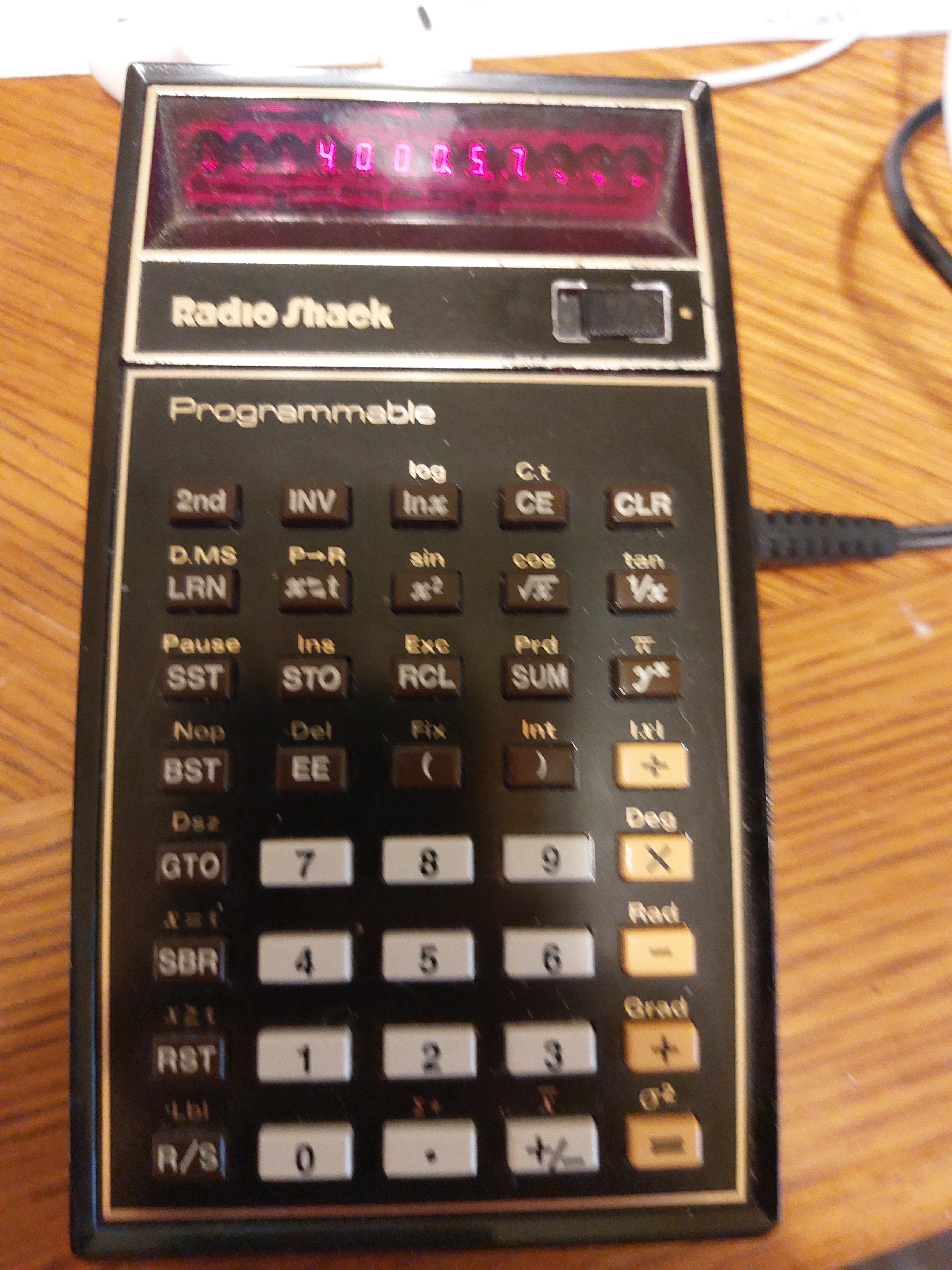
Radio Shack EC-4000 (equiv. of TI-57): Program Library

Radio Shack EC-4000 (equiv. of TI-57):   Program Library


Radio Shack EC-4000/TI-57:  Horner's Method


Let's start with a demonstration of Horner's Method, which allows a quick evaluation of polynomials.   For a quadratic polynomial:


p(x) = a * x^2 + b * x + c = x * (a * x + b) + c


The program demonstrates an example polynomial:


p(x) = 3 * x^2 - 4 * x + 9 = x * (3 * x -  4) + 9


Step:  Key Code [ Key ]

00: 32, 1 [ STO 1 ]

01:  55 [ × ]

02:  03  [ 3 ]

03:  65  [ - ]

04:  04 [ 4 ]

05:  85  [ = ]

06:  55 [ × ]

07:  33, 1 [ RCL 1 ]

08:  75  [ + ]

09:  09  [ 9 ]

10:  85 [ = ]

11:  81  [ R/S ]

12:  71  [ RST ]


Examples:

p(0) = 9

p(5) = 64

p(9) = 216


Horner's Method can apply to higher order polynomials.  


Radio Shack EC-4000/TI-57:  Permutation and Factorial


This is to add two of the common probability functions that are missing with on the calculator.  


nPr = n! / (n - r)!


If n = r, then nPn = n!


Store n in R0 (register 0), r in R1 (register 1), then run the program (RST, R/S).


Other registers used:  R2:  nPr,  R7:  n-r+1 


Note that R7 is also the t-register.  


Step:  Key Code [ Key ]

00:  01  [ 1 ]

01:  32, 2  [ STO 2 ]

02:  33, 0  [ RCL 0 ]

03:  65   [ - ]

04:  33, 1  [ RCL 1 ]

05:  75  [ + ]

06:  01  [ 1 ]

07:  85  [ = ]

08:  32, 7 [ STO 7 ]

09:  86, 5 [ LBL 5 ]

10:  33, 0 [ RCL 0 ]

11:  39, 2  [ Prd 2 ]

12:  01  [ 1 ]

13:  -34, 0 [ INV SUM 0 ]

14:  33, 0 [ RCL 0 ]

15:  76  [ x≥t ]

16:  51, 5 [ GTO 5 ]

17:  33, 2 [ RCL 2 ]

18:  81  [ R/S ]

19:  71  [ RST ]


Examples:

n = 6, r = 6:  6P6 = 6! = 720

n = 5, r = 3:  5P3 = 60

n = 11, r = 6:  11P6 = 332,640

n = 52, r = 5:  52P5 = 3.118752 * 10^8


Radio Shack EC-4000/TI-57:  Snell's Law


There are two subroutines in this program listing.  Subroutines accessed by the [ SBR ] key.  


Snell's Law describes, among other things, the relationship between index of refraction of a medium (n) and refraction angle of the direction of light (Θ) is stated by:


n1 * sin(Θ1) = n2 * sin(Θ2)


Subroutine 1:  Solve for n2.  n2 = (n1 * sin(Θ1)) / sin(Θ2)


Subroutine 2:  Solve for Θ2.  Θ2 = arcsin( n1 * sin(Θ1) / n2 )


The registers used are:  R1 = n1, R2 = n2,  R3 = Θ1, R4 = Θ2


Step:  Key Code [ Key ]


// Solve for n2

00:  86, 1  [ LBL 1 ]

01:  50  [ DEG ]

02:  33, 1 [ RCL 1 ]

03:  55  [ × ]

04:  33, 3  [ RCL 3 ]

05:  28  [ SIN ]

06:  45  [ ÷ ]

07:  33, 4 [ RCL 4 ]

08:  28  [ SIN ]

09:  85  [ = ]

10:  32, 2 [ STO 2 ]

11:  81  [ R/S ]


// Solve for Θ2

12:  86, 2  [ LBL 2 ]

13:  50  [ DEG ]

14:  33, 1 [ RCL 1 ]

15:  55  [ × ]

16:  33, 3 [ RCL 3 ]

17:  28  [ SIN ]

18:  45  [ ÷ ]

19:  33, 2 [ RCL 2 ]

20:  85 [ = ]

21:  -28  [ INV SIN ]

22:  32, 4 [ STO 4 ]

23:  81 [ R/S ]


Examples:


Solve for n2:  n1 = 1.000293 (air), Θ1 = 30°, Θ2 = 19°

1.000293 STO 1

30 STO 3

19 STO 4

GSB 1

Result:  n2:  1.5362267


Solve for Θ2:  n1 = 1.000293 (air), Θ1 = 30°, n2 = 1.333 (water)

1.000293 STO 1

30 STO 3

1.333 STO 2

GSB 2

Result:  Θ2:  22.036902


Radio Shack EC-4000/TI-57:  Pseudorandom Number Generation


This program attempts to generate random numbers using the generator:


x_n+1 = frac(997 * x_n + π)


The random numbers are between 0 and 1.  An initial seed will be required 


The calculator does not have fraction and integer parts, so they have to be simulated:


int(x) ≈ x + 1E10 - 1E10

frac(x) = x - int(x), will require a register 


See steps 10 to 23.  


Due to the internal 10 digits and the simulations, expect possible roundoff errors as random numbers are continuously generated.  


Step:  Key Code [ Key ]

00:  55 [ × ]

01:  09  [ 9 ]

02:  09  [ 9 ]

03:  07 [ 7 ]

04:  75  [ + ]

05:  30  [ π ]

06:  85  [ = ]

07:  32, 6 [ STO 6 ]

08:  75  [ + ]

09:  01  [ 1 ]

10:  42  [ EE ]

11:  01  [ 1 ] 

12:  00 [ 0 ]

13:  65  [ - ]

14:  01  [ 1 ]

15:  42  [ EE ]

16:  01  [ 1 ] 

17:  00 [ 0 ]

18:  85 [ = ]

19:  -42  [  INV EE ]

20:  -34,6  [ INV SUM 6 ]

21:  33, 6 [ RCL 6 ]

22:  81  [ R/S ]

23:  71  [ RST ]


Example:


Seed:  0.98

Generation:

0.2015927

0.1294647

0.2178986

0.3864470

0.4292517


Until next time,


Eddie 


All original content copyright, © 2011-2023.  Edward Shore.   Unauthorized use and/or unauthorized distribution for commercial purposes without express and written permission from the author is strictly prohibited.  This blog entry may be distributed for noncommercial purposes, provided that full credit is given to the author. 


Earth's Radius by Latitude

Earth's Radius by Latitude Introduction: Calculating the Earth’s Radius In quick, general calculations, we assume that the...