HP Prime Basic Planetary Data

HP Prime Basic Planetary Data

The program PLANETS and PLANETDATA retrieve data about our solar system planets, including our dwarf planet, Pluto. 

PLANETS presents you with a choose menu which will present a screen of all the data for a planet.

PLANETDATA allows you to retrieve a specific item for a planet.  PLANETDATA has two arguments:  n for the planet, k for the data point.  This is useful if you want to pull out a specific data point for calculations.

Table for PLANETDATA(n, k):                              

Value	Planet (n)	Data Point (k)
1	Mercury	Name of the Planet
2	Venus	Radius (km)
3	Earth	Mass (kg)
4	Mars	Gravity (m/s^2)
5	Jupiter	Density (g/cm^3)
6	Saturn	Axial tilt (°)
7	Uranus	Period (days)
8	Neptune	Number of Moons
9	Pluto (dwarf planet)

Example:

The gravity on Mars.  PLANETDATA(4,4) returns 3.71 m/s^2.

The diameter of Saturn.  PLANETDAT(6,2) returns 58,232 km.

HP Prime Program:  PLANETS

EXPORT PLANETS()

BEGIN

// Solar System Data

// solarsystem.nasa.gov

// EWS 2016-09-25

LOCAL head, data, n, k, str;

head:={"Planet","Radius (km)",

"Mass (kg)","Gravity (m/s^2)",

"Density (g/cm^3)",

"Axial tilt (°)",

"period (days)",

"# Moons"};

data:={{"Mercury",2439.7,

3.30104ᴇ23,3.7,5.427,.034,

58.646,0},

{"Venus",6051.8,

4.86732ᴇ24,8.87,5.243,177.36,

243.018,0},

{"Earth",6371,

5.9722ᴇ24,9.80665,5.513,23.4393,

365.24,1},

{"Mars",3389.5,

6.4169ᴇ23,3.71,3.934,25.19,

687,2},

{"Jupiter",69911,

1.89813ᴇ27,24.79,1.326,3.1,

4332.59,67},

{"Saturn",58232,

5.68319ᴇ26,10.4,.687,26.7,

10759.22,62},

{"Uranus",25362,

8.68103ᴇ25,8.87,1.27,97.8,

30688.5,27},

{"Neptune",24622,

1.0241ᴇ26,11.15,1.638,28.3,

60182,14},

{"Pluto",1151,

1.3090ᴇ22,0.66,2.05,122.53,

90560,5}

};

CHOOSE(n,"Planet",{"Mercury","Venus",

"Earth","Mars","Jupiter","Saturn",

"Uranus","Neptune"});

// Print Screen

PRINT();

FOR k FROM 1 TO SIZE(head) DO

str:=head(k)+": "+data(n,k);

PRINT(str);

END;

RETURN "Done.";

END;

HP Prime Program: PLANETDATA

EXPORT PLANETDATA(n,k)

BEGIN

// Solar System Data

// solarsystem.nasa.gov

// Individual data

// Get data on the fly

// EWS 2016-09-25

LOCAL head, data;

head:={"Planet","Radius (km)",

"Mass (kg)","Gravity (m/s^2)",

"Density (g/cm^3)",

"Axial tilt (°)",

"period (days)",

"# Moons"};

data:={{"Mercury",2439.7,

3.30104ᴇ23,3.7,5.427,.034,

58.646,0},

{"Venus",6051.8,

4.86732ᴇ24,8.87,5.243,177.36,

243.018,0},

{"Earth",6371,

5.9722ᴇ24,9.80665,5.513,23.4393,

365.24,1},

{"Mars",3389.5,

6.4169ᴇ23,3.71,3.934,25.19,

687,2},

{"Jupiter",69911,

1.89813ᴇ27,24.79,1.326,3.1,

4332.59,67},

{"Saturn",58232,

5.68319ᴇ26,10.4,.687,26.7,

10759.22,62},

{"Uranus",25362,

8.68103ᴇ25,8.87,1.27,97.8,

30688.5,27},

{"Neptune",24622,

1.0241ᴇ26,11.15,1.638,28.3,

60182,14},

{"Pluto",1151,

1.3090ᴇ22,0.66,2.05,122.53,

90560,5}

};

IF n==0 THEN

RETURN head;

ELSE

RETURN data(n,k);

END;

END;

Sources:

NASA Solar System Exploration.  https://solarsystem.nasa.gov/

Wikipedia. https://en.wikipedia.org/wiki/Main_Page

We pages retrieved during September 21, 2015 to September 25, 2015

This blog is property of Edward Shore, 2016.

HP Prime: Mathematical Calculations with 3-Dimensional Vectors

HP Prime:  Mathematical Calculations with 3-Dimensional Vectors

Note: all examples are calculated in Degrees mode.

Rectangular to Spherical Coordinates

The program RECT2SPH converts the coordinates [x, y, z] to [r, θ, ϕ].

Syntax:  RECT2SPH([x, y, z])

HP Prime RECT2SPH:  Rectangular to Spherical Coordinates

EXPORT RECT2SPH(v)

BEGIN

// [x,y,z]→

LOCAL r,θ,φ,x,y,z;

x:=v(1); y:=v(2); z:=v(3);

r:=√(x^2+y^2+z^2);

θ:=ATAN(y/x);

φ:=ACOS(z/r);

RETURN [r,θ,φ];

END;

Example:  RECT2SPH([2, 3, 4]) return [5.38516480713, 56.309932474, 42.0311137741]

Spherical to Rectangular Coordinates

The program SPH2RECT converts the coordinates [r, θ,  φ] to [x, y, y].

Syntax:  SPH2RECT([r, θ,  φ])

HP Prime SPH2RECT:  Spherical Coordinates to Rectangular Coordinates

EXPORT SPH2RECT(v)

BEGIN

// [r,θ,φ]→

LOCAL r,θ,φ,x,y,z;

r:=v(1); θ:=v(2); φ:=v(3);

x:=r*COS(θ)*SIN(φ);

y:=r*SIN(θ)*SIN(φ);

z:=r*COS(φ);

RETURN [x,y,z];

END;

Example:  SPH2RECT([6, 30, 48]) returns [3.86149378532, 2.22943447643, 4.01478363815]

Linear Distance

The program LIN3DIST is the linear distance between two three-dimensional points.  The coordinates are Cartesian.  Enter each coordinate point separately. 

Syntax:  LIN3DIST(x1, x2, y1, y2, z1, z2)

HP Prime LIN3DIST:  Linear distance between coordinates

EXPORT LIN3DIST(x1,x2,y1,y2,z1,z2)

BEGIN

// linear distance

LOCAL d;

d:=√((x2-x1)^2+(y2-y1)^2

+(z2-z1)^2);

RETURN d;

END;

Example:  Find the linear distance between points (2,3,-7) and (-1,8,2).

Input:  LIN3DIST(2, -1, 3, 8, -7, 2) returns 10.7238052948.

Spherical Distance (Arc Length)

The program SPH3DIST is the spherical distance between two three-dimensional points that share the same radius.  This is similar to the great circle distance.

Syntax:  SPH3DIST(r, φ1, φ2 ,λ1 ,λ2)

HP Prime SPH3DIST:  Spherical distance between coordinates

EXPORT SPH3DIST(r,φ1,φ2,λ1,λ2)

BEGIN

// Spherical Distance

LOCAL d;

d:=ACOS(SIN(φ1)*SIN(φ2)+

COS(φ1)*COS(φ2)*COS(λ1-λ2));

d:=d*r;

RETURN d;

END;

Example:  Find the spherical distance between points φ1 = 40°, φ2 = 64°, λ1 = -18°, λ2 = 33°.  The radius is 14.

SPH3DIST(14, 40, 64, -18, 33) returns 519.226883434

   

Angle between Two Three-Dimensional Coordinates

The program VANGLE calculates the angle between two points.  Both points are entered in vector form.

Syntax:  VANGLE([x1,y1,z1], [x2,y2,z2])

HP Prime VANGLE:  Angle between two coordinates

EXPORT VANGLE(v1,v2)

BEGIN

// Angle between 2 vectors

LOCAL θ;

θ:=ACOS(DOT(v1,v2)/

(ABS(v1)*ABS(v2)));

RETURN θ;

END;

Example:  Find the angle between [5,4,5] and [2,0,-3]. 

VANGLE([5,4,5],[2,0,-3]) returns 99.8283573577°

Rotating a Cartesian Coordinate Vector

The program ROT3X, ROT3Y, and ROT3Z rotates the three-dimensional vector [x, y, z] with respect to the x-axis (ax),  respect to the y-axis (ay), and respect to the z-axis (az), respectively.

Syntax:  ROT3X(v, ax),  ROT3Y(v, ay),  ROT3Z(v, az)

Caution:  the result will be a matrix instead of a vector

HP Prime: ROT3X

EXPORT ROT3X(v,ax)

BEGIN

// [x,y,z],θx

v:=TRN(v);

v:=[[1,0,0],[0,COS(ax),−SIN(ax)],

[0,SIN(ax),COS(ax)]]*v;

RETURN TRN(v);

END;

HP Prime:  ROT3Y

EXPORT ROT3Y(v,ay)

BEGIN

// [x,y,z],θy

v:=TRN(v);

v:=[[COS(ay),0,SIN(ay)],

[0,1,0],[−SIN(ay),0,COS(ay)]]*v;

RETURN TRN(v);

END;

HP Prime:  ROT3Z

EXPORT ROT3Z(v,az)

BEGIN

// [x,y,z],θz

v:=TRN(v);

v:=[[COS(az),−SIN(az),0],

[SIN(az),COS(az),0],[0,0,1]]*v;

RETURN TRN(v);

END;

Example:  Rotate the vector [2, 3, 4] 30°, with respect to the x-axis, y-axis, and z-axis, separately and respectfully.

ROT3X([2, 3, 4], 30) returns [[ 2, 0.598076211352, 4.96410161514 ]]

ROT3Y([2, 3, 4], 30) returns [[ 3.73205080757, 3, 2.46410161514 ]]

ROT3Z([2, 3, 4], 30) returns [[ 0.232050807568, 3.59807621135, 4]]

This blog is property of Edward Shore, 2016

HHC 2016 Highlights

HHC 2016 Highlights

When:  September 17 and 18, 2016

Where: Fort Collins, CO

If you are a fan of Hewlett Packard calculators and math, the annual HHC conferences, held every September, could be a weekend conference for you.  I have attended HHC conferences since 2003 and went most years.  

Here some highlights from this years’ conference.  You can access the presentations here:  http://hhuc.us/2016/files/Speakers/.  Also with each section, the youtube of each talk is now available as of today (Thank you Eric Rechlin of hpcalc.org!)

 

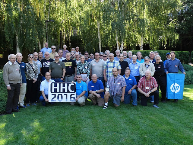The HHC 2016 Group Photo - Used by Permission from Jake Schwartz - Thank you!

 

First Day:  September 17, 2016

HP Calculator Power Supplies:  Jim Johnson

Video:  https://www.youtube.com/watch?v=lIjQn9a5n3U

For batteries to work for calculating devices, the batteries must provide power to last (at least a few months of use), comply with all the regulations (FCC, etc), fit in a small space, and if the batteries are rechargeable, they must be able to recharge safely.  The area of where batteries can be used safely is small.  For lithium ion batteries, the range is between 2 and 4 volts, operating between 0°C and 100°C.  Battery problems caused Samsung Galaxy 7 phone and hover boards to be recalled.  

The original HP 35 (1972) power supply worked with 4 different voltages.  A similar power supply used for the HP 29C (1977).  As we can imagine, as calculators grow complex, so do their power supply structures.  For the current HP Prime, the power supply works with 10 different voltages.  

From the HP-35 to HP 9825:  Don Morris

Video:  https://www.youtube.com/watch?v=iQdtk3pk86M

We are appreciative of Don Morris, who was one of the engineers who worked with the HP 35 and HP 9825.  

To recall the HP 35 story, idea of the HP 35 was Bill Hewett’s desire to have a pocket version of the HP 9100.  There were two plants, Palo Alto, CA and Loveland, CO, involved with the project.  A desktop prototype was worked on in Loveland, where the hand held was developed in Palo Alto.  Hewett set the price of the HP 35 at $395.  

After the HP 35, the HP 9805A, and their successors HP 45 and HP 46 were in production, there were reports HP 9805A had power problems.  Morris found a bug that caused the HP 9805A did not always powered on, the cause was a C&T chip.  The company fixed the machines but quietly.

Morris also was involved with the HP 9825A, along with Barney Oliver and Dorian Shainin.  The HP 9825A was different from the 35, 45, and 46:  it wasn’t RPN but algebraic (equations were evaluated as they were written, with implicit multiplication allowed for one-letter upper case variables). 

Morris was involved with a problem with 9825A.  A scientists in Australia was using the 9825 as part of a high altitude experiment.  A fuse went out, and in consultation, Morris suggested a ten ampere fuse, which was normally not recommended for 9825A.   Thankfully the suggestion worked.  

Calculator Bibliography Update:  Felix Gross

Video:  https://www.youtube.com/watch?v=LrkTSTo4h2I

Gross is currently putting together a list of calculator documents.   As of 2016, the list of entries grew to 4,032, and Gross is asking for references, specifically on the subject of teaching, electrical engineering, civil engineering, and finance.  His email is felix.gross@alumni.ethz.ch .  Gross has noted the publishing of calculator peaked around 1980 and 1981.  

Raspberry PI Update:  Jackie Woldering

Video:  https://www.youtube.com/watch?v=2OeSRVhqCHA

 

The Raspberry PI, a low cost computer which runs on Linux, has taken off.  Current models include Model A+, Model B, and Raspberry Pi Zero.  The base model is the Raspberry Pi Zero, it has mini-HDMI port, one micro USB port, and is used either a stand-alone or used for embedded design.  The Zero model has 1 GHz single-core processor with 512 MB RAM, and is currently sold for $5.  

As I will mention later, I won a model Zero as a door prize and look forward to learning about Linux.  

The most advanced model is the Raspberry Pi 3 Model B, which features a 1.2 GHz 64-bit quad-core ARM processor, wireless port, 1 GB RAM, 4 USB ports, Bluetooth, and Wifi.  This can be yours for $35.

Software includes Python, Sonic Pi, a music software, and games.  

Website:  https://www.raspberrypi.org/

 

Calculation Tricks: Namir Shammas 

Video:  https://www.youtube.com/watch?v=YYOc5GRK6do

We are always looking for ways to cut computing time down while keeping (or even approving) computational accuracy.  Namir Shammas is an expert in calculator programming and computation.  Here are some of the tips shared:

Calculating Derivatives:  You can adjust the step size, h, automatically (instead of asking for the user to input h) by using the following adjustment:  h = 0.01*(1 + |x|).

Newton’s Method:  Avoid dividing by zero in your steps by replacing the recurring step with:

x_n+1 = x_n * ( f(x_n) * f’(x_n) ) / ( f’(x_n)^2 + E ),  where E is an arbitrary small number that you provide. 

Primes can be found by using the Solovay-Strassen Primality Test and Miller-Rabin Primality Test. 

You can normalize regression data (reign in data with large ranges) to the range [a, b] by the following formula: 

( (x – x_min) / (x_max – x_min) ) * (b – a) + a

The user can choose the values of a and b.  Namir suggests that a = 1 and b = 2.  Calculate regression.  Don’t forget to translate back to the appropriate values.

Next Generation Calculation Measurement: Richard Nelson

Video:  https://www.youtube.com/watch?v=9ukvU3KcfzQ

Key factors in measuring calculator power include current drain of the power, the required power to operate a calculator, how to troubleshoot component, and how the power confirm to specs.  Nelson demonstrated a power measurement with a Mooshimeter.  The Mooshimeter is a compact meter that measures voltage, current, resistance, and temperature.  The kicker is that the Mooshimeter does not have a display, thus it would have to connected to a computer in order to read results.  

HP 41CL Update: Gene Wright

Video: https://www.youtube.com/watch?v=FrgGxT59YE4

An ultimate version of the HP 41C is the HP 41CL.  The HP 41CL contains nearly all the functions of the HP 41C, its available ROMs (except the time module), with other extended commands and functions.   Most HP 41Cs can be turned into a HP 41CL by replacing its original CPU board.  Talk about expanding the life of the HP 41C, which first came into our calculator community in 1979.  

Should you have one (or buy one, which will cost you about $250), there are new updates for the HP 41CL, such as:

PowerCL Extreme:  additional alpha functions (MID$, LADEL, CLA? (clear alpha?)), flag toggle functions, set and clear flags indirectly  (SFX, CFX)

Total Rekall:  Stack shuffle commands and other stack selection commands

CL Expanded Memory Rom:  has the stack swap functions from Total Rekall plus room to run four “copies” of the 41C on the same device

Greg J McClure’s Rom:  additional math utilities, probability distributions, and slide rule functions

HP 67/97 Games Rom:  Most of the games that were programmed for the HP 67 and HP 97.  

The HP 41CL web page:  http://www.systemyde.com/hp41/index.html

 

HP-41CL ROM Database:  Syvlain Cote

Video: https://www.youtube.com/watch?v=9eWwXbLwgo8

Cote demonstrates updating a HP 41CL.  The ROM can be updated one image at time, or all eight pages at once.  

3D Printing and Machine with the HP Prime:  Jim Donnelly

Video:  https://www.youtube.com/watch?v=MN0BStwuDug

Donnelly dedicated his talk to Don Morris.  I am a fan of 3D printers and amazed of what they produce.  Donnelly express that the HP Prime should be able to not only express 3D graphs but also generate 3D printer files that will be used as programs used in the printer.

There are two printing files: CNC and STL.  CNC files describes how the cutting tools act, while STL files describe what is to be printed.  Challenges include the natural files and limits of what can be stored in strings and lists.

Donnelly created several HP Prime programs to assist the printer in creating CNC files (ReadPrimeList, WriteColumnUp) and STL files (MAKEVERTEX, FMT).  

Merely talking about it just doesn’t do it justice, to see the programs and results, please see the presentation (by Jim Donnelly) in the HHC 2016 link provided at the beginning of this blog entry or the video above.   

New RPL:  Gunter Schinck

Video:  https://www.youtube.com/watch?v=YxN49QDHQMM\

The HP 50g may no longer be in production (production has ceased in 2015), but that doesn’t stop us enthusiasts from programming and improving on the 50g infrastructure. 

The author of the New RPL is Claudio L., which is an HPGCC3 project.  Website:  http://hpgcc3.org/  

Some features of New RPL (which is still a work in progress, according to the website, it is about 25%):

* Increase in speed processing, from 4.6 times faster (than a normal HP 50g) for complex functions to 60 times faster for basic arithmetic.

* In list processing the functions of [ + ] and ADD are reversed from the HP 50g practice.

* There are six more soft keys, mapped to the [APPS], [MODE]. [TOOL], [VAR], [STO>], and [NXT] keys.  Affected functions are moved elsewhere.  For example, Undo is moved to the left key, copying and pasting modes are also mapped to the left key (by use in combination with the left-shift key), and the [HIST] key now house store and recall.

* Pressing and holding [ ON ] with [SPC] toggles with format setting (STD, FIX, SCI, ENG).  Holding [ON[ with a number key gives the decimal place setting.

* Numbers in NewRPL can have exponents up to 3000 instead of just 499.

* With the degree and radian tags, the grads and DMS (degree minutes second) angle tags have been added.

Second Day:  September 18, 2016

DM 42:  Gunter Schinck

Video:  https://www.youtube.com/watch?v=bU-_9x8dEM8

Swiss Micros (www.swissmicros.com) is known for creating credit card size (and for some, larger landscape) versions of the HP 11C (DM 11), 12C (DM 12), 41C (DM 41), 15C (DM 15), and 16C (DM 16).  In the works is a recreation of the HP 42S currently named the DM 42P.  While still smaller than the HP 42S, the DM 42P would be an enhanced 42S.   Improvements include a USB port, a clock, SD slot (backup), 128KM RAM, 5 MB flash, and alpha keys moved to the keypad.  The proposed screen would become larger, from 2 lines to 6 lines, one will be used for the soft menu.  The DM 42 will run on Thomas Oakken’s Free42.  Swiss Micros plans to release the DM 42S in late 2016 (it could be possible the official release takes place in 2017).    

This video from Michael Steinmann of Swiss Micros shows a rendering of what the DM 42P will look like:  https://www.youtube.com/watch?v=qxZQQkh_8Og&feature=youtu.be  

Even More RAM with FRAM71B:  Bob Prosperi

Video:  https://www.youtube.com/watch?v=64CqEF27BoU

The HP 71B keeps getting new life.  As the slogan “Now you can cram even more RAM, with FRAM”, the FRAM71B upgrades the memory to a base 512 KB (which can be doubled), allow two “copies” of the 71B to work in the same machine, lowers the power consumption in sleep mode, and adds the FORTH/Assembler and HP-41 Translator ROMs.  Propsperi details the development of the FRAM71B and how the software would be installed with into the HP 71B.  

The new FRAM71B boards are limited in availability, see this thread for details for availability and cost:  http://hpmuseum.org/forum/thread-5437.html

 

HP-01 “Cricket”:  Geoff Quickfall 

Video:  https://www.youtube.com/watch?v=2RE3-xsbyb0

In addition to being an air pilot, Quickfall is the go-to man when it comes to restoring and repairing classic technology.  Quickfall talks about repairing the class HP-01 watch and installing a repair kit, created by Berhard Emese.  The repair not restores the watch but gives additional features:  extended battery life and two hundred year calendar range (1900-2099).  

Link to the repair kit:  http://www.panamatik.de/html/hp-01_repair_kit.html   

The talk concludes with the HP 25E/19E ACTs, which updates any HP Woodstock series calculators (1970s).

Final comment:  I have got to believe that wearing a HP-01 in the late 1970s made you the hit of the discotheques. 

HP 71B Compendium:  Sylvain Cote

Video:  https://www.youtube.com/watch?v=Jk6ZoW6dxqU

Cote’s compendium lists all the documents associated with the HP 71B (including mods, product ROMs, overlays, manuals, etc).  

It is being updated, but here is a link to the 2015 compendium:  http://www.hpmuseum.org/forum/thread-5286.html   

HP Prime Regression Model Selection:  Namir Shammas

Video: https://www.youtube.com/watch?v=hcskiz3fdE0

The talk was dedicated to Jon Johnson, who was the curator of the HP Computer Museum website (http://hpmuseum.net/).  Rest in peace, Johnson. 

The best fit programs is based on the best fit linearized programs for the HP 65, HP 67, and the PPC ROM.  

Generally, two data sets are used, one called a training set and one for a data set, with each set having different noise (unexplained variations).    For each model tested, the following are calculated:  slope, intercept, and the MSSE (mean square sum of errors) for both the training and data set along with a weighted average.  From the calculations, the model with the best fit is selected.  The programs featured at Best_YX_LR_Machine_Learning_1.txt and Best_YX_LR_Machine_Learning_2.txt, the latter used normalized values.

For details and programming, please check out Shammas’ talk about curve fitting (see the link to the talks about the beginning of this blog entry).

In Praise of the SR-56 Calculator:  Gene Wright

Video:  https://www.youtube.com/watch?v=oDtWB5ebssw

This talk is a comparison of the Texas Instruments SR-56 (1976) and the HP-25 (C) calculators.  

Regarding the SR-56 and HP-25:

* The SR-56 had 100 partially merged steps (steps only merged with the [2^nd] key).  The HP 25C only had 49 steps, but they were fully merged (with the [ f ], [ g ], [ STO ], storage arithmetic, and [ RCL ] keys).

* There were 10 data registers available at all times on the SR-56, while the HP-25 only had eight. 

* For comparisons, the SR-56 used an independent t register, while the HP-25 used the x and y stacks. 

* The SR-56 had a [2^nd] [LRN] (f(n)) sequence that allowed access to the Σ+, Σ-, mean, standard deviation, and rectangular/polar conversions.  This was the only way these functions could be accessed.

* Unique to the SR-56 were subroutines, DSZ (decrease by 1, skip on 0), and pause.  Unique to the HP 25C were a low battery warning, % key, H to HMS conversion, and engineering mode.

Programming Contests

Every year there are two programming contests.  They may be over but you can check them out right here:

RPL (HP 48, 49, 50):  http://www.hpmuseum.org/forum/thread-6871.html

RPN (WP-34): http://www.hpmuseum.org/forum/thread-6870.html

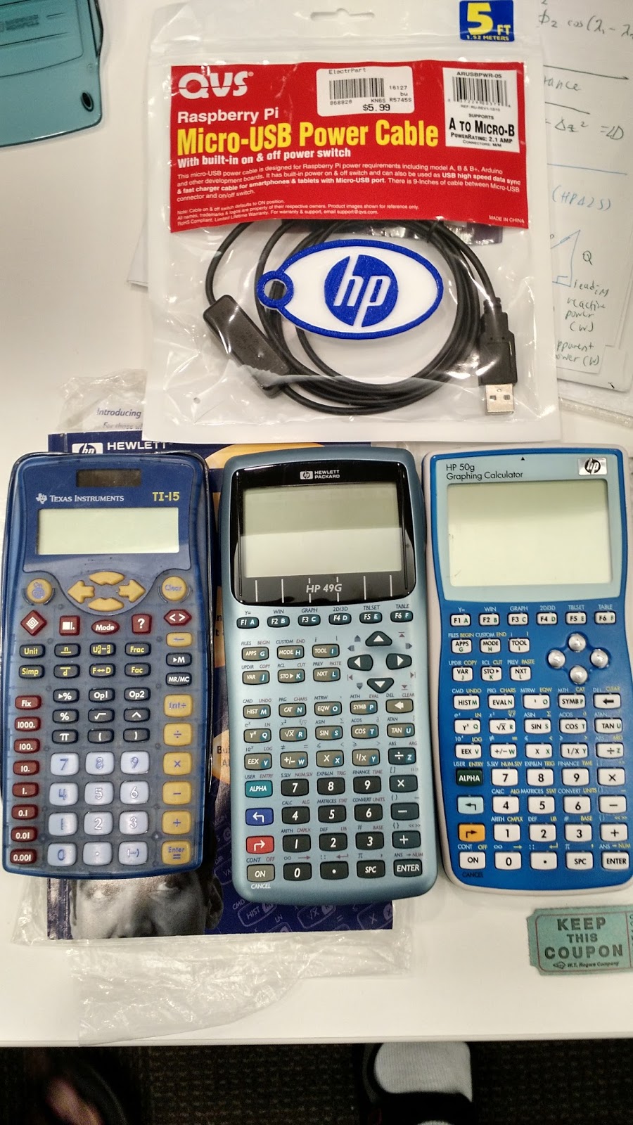
Door Prizes 

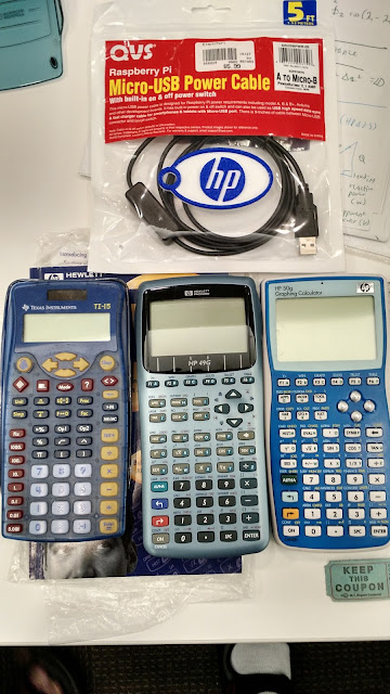My Haul:  Raspberry PI (top), TI-15 (left), HP 49G (center).   The HP 50g I already had.

 

There was enough door prizes to go around that everyone left with at least three items each.  I donated an HP-50g (black keyboard) and a Calculated Industries Real Estate II.   I did pretty well for the door prizes:  HP 49G (not 49g+, instead the blue keyboard which to my surprise is really good), TI-15, and a Raspberry Pi Zero (a Linux computer).

Plans for HHP 2017

If you get a chance and you are a fan of calculators (particularly Hewlett Packard), I encourage you to attend.  The next conference is scheduled to be on September 16-17, 2017, place to be determined.  As we get closer to next September, more details will be worked out.

I want to do a presentation for the conference, right now one of two topics I am thinking of are talking about my blog or fast tips and tricks for the HP 12C.  Of course, this is all subject to change.

Until next time, have a great and wonderful day,

Eddie

This blog is property of Edward Shore, 2016