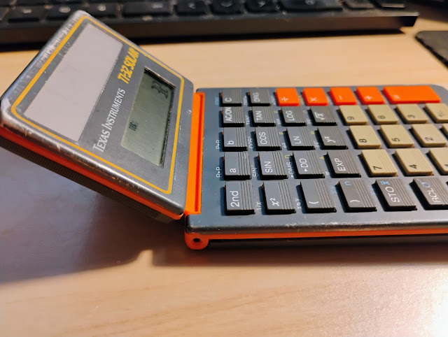
Spotlight: TI-32 Solar from 1988

Spotlight: TI-32 Solar from 1988

Today’s spotlight is on a standard scientific calculator from Texas Instruments… with a twist. First, let’s start with the quick facts.

Quick Facts

Model: TI-32 Solar

Company: Texas Instruments

Timeline: 1988 (possibly 1989?), this model was very short lived

Type: Scientific

Memory: 1 memory register

Power: Solar

Screen: 10 digits

The TI-32 Solar was a scientific calculator that was sold briefly by Texas Instruments in the last 1980s. The function set is a combination of the TI-30 Solar and the original one line TI-34:

* trigonometry, decimal/dms conversion, rectangular/polar conversions

* logarithms, anti-logarithms (10^x, e^x), powers

* one variable statistics (mean, deviation, sums)

* binary/decimal/hexadecimal conversion (and just conversions, strangely no octal)

* 3-decimal random number generator (RND)

* percent function

The Polar/Rectangular conversions use the [ a ] and [ b ] keys. [ a ] is for x and r, while [ b ] is for y and Θ.

The statistics mode is one-variable only. Though I am not a fan of the STAT mode being the alternative function of the [ C ] key, thankfully, the stat mode works.

What truly sets the TI-32 Solar apart are two things:

(1) The orange trim and keys on a dark gray keyboard. This is a very rare color scheme, especially orange until Texas Instruments started to release the TI-30XIIS and the TI-84 Plus CE in various colors.

(2) The screen tilts. The screen is a set on a hinge that allows the user to tilt the screen to different angles, which allows for more ergonomic operation. To put the calculator away, tilt the screen to be aligned with the keyboard and use the slide case. I think this is a really neat idea. The tilt mechanism seems to hold out well for a nearly 40 year old calculator.

Source

Woerner, Joerg. “Texas Instruments TI-32 SOLAR” Datamath Calculator Museum. September 20, 2002. Accessed July 7, 2025. http://www.datamath.org/Sci/Modern/TI-32Solar.htm

Eddie

 All original content copyright, © 2011-2025. Edward Shore. Unauthorized use and/or unauthorized distribution for commercial purposes without express and written permission from the author is strictly prohibited. This blog entry may be distributed for noncommercial purposes, provided that full credit is given to the author.

All posts are 100% generated by human effort.  The author does not use AI engines and never will.

HP 21S and TI-84 Plus CE: Normal Distributions and Hypothesis Tests

HP 21S and TI-84 Plus CE: Normal Distributions and Hypothesis Tests

Let’s compare how calculations involving the normal distribution are done between a classic calculator and a current one. The classic calculator is the rare HP 21S calculator from 1988 and the current calculator is the TI-84 Plus CE.

In 2017 (how time flies!) I wrote a review for the HP 21S (along with it’s cousin HP 20S):

https://edspi31415.blogspot.com/2017/04/retro-review-hewlett-packard-hp-20s-and.html.

Normal Distribution Calculations

z = z-score, point; p = probability, area

Assumptions: The mean is assumed to be 0 while the standard deviation is 1. (μ = 0, σ = 1).

Lower Tail (-∞, z)

	HP 21S	TI-84 Plus CE*	Example
Given z, find p	Keystrokes: 1 [ - ] z [ ←| ] (Q(z)) [ = ]	normalcdf(-1E99, z)	Input: z = 0.77 Result: p ≈ 0.7794
Given p, find z	Keystrokes: [ ( ] 1 [ - ] p [ ) ] [ |→ ] (zp)	invNorm(p)	Input: p = 0.77 Result: z ≈ 0.7388

* also includes TI-83 Plus, TI-84 Plus, TI-83 Premium (Python), TI-82 Advanced, and I do believe it is the same syntax for TI-89/Nspire family

Upper Tail (z, +∞)

	HP 21S	TI-84 Plus CE*	Example
Given z, find p	Keystrokes: z [ ←| ] (Q(z))	normalcdf(z, 1E99)	Input: z = 0.49 Result: p ≈ 0.3121
Given p, find z	Keystrokes: p [ |→ ] (zp)	InvNorm(1 - p)	Input: p = 0.49 Result: z ≈ 0.0251

Two Tail (-z, z)

	HP 21S**	TI-84 Plus CE*	Example
Given z, find p	Keystrokes: z [ STO ] [ 0 ] [ +/- ] [ ←| ] (Q(z)) [ - ] [ RCL ] 0 [ ←| ] (Q(z)) [ = ]	normalcdf(-z, z)	Input: z = 1 Result: p ≈ 0.6827
Given p, find z	Keystrokes: p [ ÷ ] 2 [ = ] [ STO ] 0 Lower Limit: [ ( ] 0.5 [ - ] [ RCL ] 0 [ ) ] [ |→ ] (zp) Upper Limit: [ ( ] 0.5 [ + ] [ RCL ] 0 [ ) ] [ |→ ] (zp)	InvNorm(p, 0, 1, CENTER)	Input: p = 0.25 Result: Upper: z ≈ 0.3186 Lower: z ≈ -0.3186

** HP 21S: A memory register is needed for this particular algorithm. I use register 0 for this example.

Sample Test of the Mean: Is the Proposed Mean the True Mean? (μ0 = μ)

Perform a significant test of whether a proposed mean (μ0) is the true mean (μ) given data from a sample:

x-bar: arithmetic mean of a sample

σ: population deviation of the sample

n: sample size

In this test, the null or default hypothesis is μ =μ0, while the alternate hypothesis is μ ≠ μ0.

Your confidence level and critical level, α, are complimentary. For example, if you want a 95% confidence level, your critical level, or α, is: α = 1 – 0.95 = 0.05 (5%). This is a two-tail test.

HP 21S	TI-84 Plus CE
[ ←| ] [ ← ] (LOAD) (A) (1-Stat) n [ XEQ ] D μ [ R/S ] σ [ R/S ] Test Method # 1: α [ ÷ ] 2 [ = ] [ |→ ] (zp) (= critical value) μ0 [ XEQ ] B (= test value) Null: μ0 = x-bar, Alternative: μ0 ≠ x-bar If test value < critical value, do not reject null hypothesis If test value > critical value, reject null hypothesis and accept the alternate hypothesis Test Method # 2: μ0 [ XEQ ] B [ ←| ] [ 1 ] (Q(z)) (= p) Null: μ0 = x-bar, Alternative: μ0 ≠ x-bar If p > α / 2, do not reject null hypothesis If p < α / 2, reject null hypothesis and accept the alternate hypothesis Note: LBL D: store summary statistics for the test of one sample mean or probability. For this test, the standard error that is shown will not be used. LBL B: calculate the z-score: z = (x-bar – μ0) / (σ / √n)	[ stat ], TESTS, 1: Z-Test… Inpt: Stats (Input shown as Inpt) μ0: enter μ0 σ: enter σ x-bar: enter x-bar n: enter n Select μ ≠ μ0 (alternate hypothesis) Select Calculate Test Method # 1: critical value: normalcdf(α/2, 1E99) test value: [ vars ], 5: Statistics…, TEST, 2: z Null: μ0 = μ, Alternative: μ0 ≠ μ If test value < critical value, do not reject null hypothesis If test value > critical value, reject null hypothesis and accept the alternate hypothesis Test Method # 2: Compare p to α Null: μ0 = x-bar, Alternative: μ0 ≠ x-bar If p > α, do not reject null hypothesis If p < α, reject null hypothesis and accept the alternate hypothesis One line command: Z-Test(μ0, σ, x-bar, n, alt) alt: -1 for μ0 < μ, 0 for μ0 ≠ μ, 1 for μ0 > μ
Example: n = 515, μ = 7.65, σ = 3.56 α = 5% = 0.05, μ0 = 7.7, α / 2 = 0.025 [ ←| ] [ ← ] (LOAD) (A) 515 [ XEQ ] D 7.65 [ R/S ] 3.56 [ R/S ] 0.05 [ ÷ ] 2 [ = ] [ |→ ] (zp) (critical value = 1.9600) 7.7 [ XEQ ] B (z ≈ -0.3187 < 1.9600) 7.7 [ XEQ ] B [ ←| ] [ 1 ] (Q(z)) (p ≈ 0.6250 > 0.025) Do not reject null hypothesis	Example: n = 515, μ = 7.65, σ = 3.56 α = 5% = 0.05, μ0 = 7.7 [ stat ], TESTS, 1: Z-Test… Inpt: Stats μ0: 7.7 σ: 3.56 x-bar: 7.65 n: 515 Select μ ≠ μ0 Select Calculate Results: μ≠7.7 z=-0.3187304977 p=0.7499310153 x-bar=7.65 n=515 p ≈ 0.7499 > 0.05 z ≈ -0.3187 < 1.9600 Do not reject null hypothesis

This is one of several z-tests that can be performed.

Confidence Interval

Determine a confidence level of where the true mean is located given data from a sample:

x-bar: arithmetic mean of a sample

σ: population deviation of the sample

n: sample size

Confidence Mean:

x-bar ± (z * σ) / √n

z: absolute value of the z-score where the two tail probability equals c.

Using TI-84 Plus CE commands: invNorm(c, 0, 1, CENTER)

HP 21S	TI-84 Plus CE
[ ←| ] [ ← ] (LOAD) (A) n [ XEQ ] D μ [ R/S ] σ [ R/S ] Confidential Interval: [ ( ] 1 [ - ] c [ ) ] [ ÷ ] 2 [ = ] [ |→ ] [ 1 ] (zp) [ XEQ ] C → precision [ R/S ] → lower limit [ R/S ] → upper limit Note: LBL C: Confidence interval precision = (z * σ) / √n lower limit = x-bar – precision upper limit = x-bar + precision	[ stat ], TESTS, 7: Zinterval… Inpt: Stats (Input is shown as Inpt) σ: enter σ x-bar: enter x-bar n: enter n C-Level: enter confidence level as a decimal Calculate One line command: ZInterval σ, x-bar, n, c
n = 389, μ = 88.84, σ = 10.25 c = 90% = 0.9 [ ←| ] [ ← ] (LOAD) (A) 389 [ XEQ ] D 88.84 [ R/S ] 10.25 [ R/S ] [ ( ] 1 [ - ] 0.9 [ ) ] [ ÷ ] 2 [ = ] [ |→ ] [ 1 ] (zp) [ XEQ ] C → 0.8548 [ R/S ] → 87.9852 [ R/S ] → 89.6948	n = 389, μ = 88.84, σ = 10.25 c = 90% = 0.9 Inpt: Stats σ: 10.25 x-bar: 88.84 n: 389 C-Level: 0.9 Result: (87.985, 89.695) x-bar = 88.84 n = 389

Sources

CalcBlog “Hypothesis Testing using Z-Test on the TI-83 Plus, TI-84 Plus, TI-89, and Voyage 200” February 6, 2011. https://www.calcblog.com/hypothesis-testing-z-test-on-ti84-ti89-graphing-calculator/ Accessed January 30, 2025.

Hewlett Packard HP-21 Stat/Math Calculator: Owner’s Manual Edition 3. June 1990.

TI-Basic Developer “The Z-Test( Command” http://tibasicdev.wikidot.com/z-test Accessed January 30, 2025.

Enjoy! Until next time,

Eddie

All original content copyright, © 2011-2025. Edward Shore. Unauthorized use and/or unauthorized distribution for commercial purposes without express and written permission from the author is strictly prohibited. This blog entry may be distributed for noncommercial purposes, provided that full credit is given to the author.

HP Prime and TI-84 Plus CE Python: Quartiles of a Data Set

HP Prime and TI-84 Plus CE Python: Quartiles of a Data Set

25^th, 50^th, and 75^th Percentiles

The following code finds five points of a list of data points:

Minimum: the data point of least value

Q1: the first quartile, known as the 25^th percentile. The first quartile is median of the lower half of the data.

Median: also known as the 50^th percentile, this is the median, or middle point of the data.

Q3: the third quartile, known as the 75^th percentile. The third quartile is the median of the upper half of the data.

Maximum: the data point of the most value

The list of data is first sorted in ascending order.

The median is determined as follows:

If the number of data points is odd: Take the number that lies in the middle.

If the number of data points is even: Take the average of the middle two numbers.

The way quartile values are determine vary depending by country and jurisdiction. The program presented uses Method 1, which is used in the United States. (see Source)

If the number of data points is odd: The data is split in half, do not include the median.

If the number of data points is even: The data is split in half.

Python File: quartiles.py, quartile.py

This script does not use any module, so it should work on every calculator that has Python, along with the full-computer editions of Python. Results are shown as floating point numbers, rounded to 5 decimal places.

This was code was made with the HP Prime emulator, and was tested on with an HP Prime, a TI-84 Plus CE Python edition, and a TI-83 Premium CE Python Edition calculator.

# quartiles program

# method 1, median divides data in half

# is used (US method)

# halfway subroutine

def halfway(l):

  n=len(l)

  # get halfway point

  # Python index starts at 0

  h=int(n/2)

  # even

  if n%2==0:

    return(l[h]+l[h-1])/2

  # odd 

  else:

    return(l[h])

print("Use list brackets. [ ]")  

data=eval(input("List of Data: "))

# length of the list

nw=len(data)

# sort the list

data.sort()

print("Sorted Data: "+str(data))

# maximum and minimum

q0=min(data)

q4=max(data)

# get sublists 

h=int(nw/2)

if nw%2==0:

  l1=data[0:h]

  l3=data[h:nw]

else:

  l1=data[0:h]

  l3=data[h+1:nw]

# list check

print("1st half: "+str(l1))

print("2nd half: "+str(l3))

  

# quartiles, q2 is the median

q1=halfway(l1)

q2=halfway(data)

q3=halfway(l3)

# set up  answer strings

txt1=["min = ","Q1 = ","median = ", 

"Q2 = ","max = "]

results=[q0,q1,q2,q3,q4]

for i in range(5):

  txt2="{0:.5f}"

  print(txt1[i]+txt2.format(results[i]))

Examples

Data Set: [1, 2, 3, 4, 5]

Min = 1.00000

Q1 = 1.50000

Med = 3.00000

Q3 = 4.50000

Max = 5.00000

Data Set: [76, 46, 49, 46, 56, 52, 59, 130, 80]

Min = 46.00000

Q1 = 47.50000

Med = 56.00000

Q3 = 78.00000

Max = 130.00000

Date Set: [55, 35, 40, 50, 60, 50, 55]

Min = 35.00000

Q1 = 40.00000

Med = 50.00000

Q3 = 55.00000

Max = 60.00000

Note: A Way to Format Numbers

To format numbers to have a set number of decimal places, use the code

{ identifier : .5f }.

The identifier can be almost anything, I usually call it 0 for the 1^st number to be formatted. The number before the “f” (floating point indicator) is the number of decimal places. For example:

2 decimal places: { identifier : .2f }

5 decimal places: { identifier : .5f }

(spaces added for readability)

The text string will need to have a .format(arg) at the end of the string.

Example code:

n = 14.758119

txt = “The rounded value is {0:.5f}”

print(txt.format(n))

returns 14.75812

Source

Wikipedia. “Quartile” Last edited on February 21, 2025. https://en.wikipedia.org/wiki/Quartile Accessed May 12, 2025.

Eddie

All original content copyright, © 2011-2025. Edward Shore. Unauthorized use and/or unauthorized distribution for commercial purposes without express and written permission from the author is strictly prohibited. This blog entry may be distributed for noncommercial purposes, provided that full credit is given to the author.

Casio fx-6500P Program Library 2025

Casio fx-6500P Program Library 2025

Last birthday, I reviewed the rare classic, the Casio fx-6500G:

https://edspi31415.blogspot.com/2024/03/spotlight-casio-fx-6500g.html

Parabola Area and Maximum Point: Program P1: Steps 114

Area Under a Parabola set up by the equation:

y = -((x – a)*(x – b)) = -x^2 + p*x – q

p = a + b

q = a * b

Cls

“-((X-A)×(X-B))”

“A”? →A

“B”? → B

A+B → P

AB → Q

-B^3 ÷ 3 + B² P ÷ 2 – Q B + A^3 ÷ 3 - A² P ÷ 2 + Q A → R

“AREA:”

R ◢

“MAX PT:”

P ÷ 2 →X ◢

-((X-A)×(X-B)) → Y

The caret symbol ^ stands for [x^y].

Example:

y = -((x + 4) * (x – 2)) = -x^2 – 2*x + 8

A = -4, B = 2

Area: 36

Maximum Point: (-1, 9)

Circular Sector: Arc Length and Sector Area: Program: P2: Steps: 59

“RADIUS”? →R

“ANG(°)”? → T

RTπ÷180 →L

RL÷2 →A

“ARC LENGTH:”

L ◢

“AREA:”

A

The degree character is generated by the [° ‘ “] key.

Example:

R = 10.5, T (angle) = 120°

Results: Arc length = 21.99114858, Area = 115.45353

Integer Division: Program: P3: Steps: 51

“INT÷”

“X>0”? →X

“M>0”? →M

Int(X÷M)→Q

X-M×Q→R

Q ◢

“REM”

R

Examples:

43 Int÷ 11 = 3 Rem 10

7263 Int÷ 1849 = 3 Rem 1716

Hint: To find out the number of steps in a single program? Simply scroll down the last character and hold down the [ MDisp ] key. Kind of neat because this works outside of programming mode. I think this key was available on most Casio graphing calculators well into the fx-7700G (single G) and fx-9700Gα (E,M,H) series in mid 1990’s.

95% Population Proportion: Program P4: Steps: 96

X successes out of population N

“95 PRCT PROP”

“X”? → X

“N”? → N

X ÷ N → P

√(P(1-P))→ M

1.959963984 M ÷ √N → H

P – H → L

L + 2H → H

“LOW:”

L ◢

“HIGH:”

H

Example:

X = 850, N = 1176

Interval:

LOW: 0.6972058859

HIGH: 0.7483723454

Interval:

Source: HP 21S Stat/Math Calculator: Owner’s Manual. Hewlett Packard. 3^rd Edition. June 1990.

Power Generated by a Wind Turbine: Program P5: Steps: 82

“WIND PWR”

“RADIUS (M)”? →R

“SPEED (M÷S)”? → V

“DENSITY”? →P

π × R² × P × V^3 ÷ 2 → W

“POWER:”

W

Example:

R = 8.18 m, V = 4.48 m/s, P = 1.2 kg/m³

Result: 11340.74989 W

Source: Sharp Electronics Corporation Conquering The Sciences: Applications for the SHARP Scientific Calculator EL-506A Sharp Corporation. Osaka, Japan. 1986. pp.75-77

Round to Nearest Integer (display only): Program P6: Steps: 11

?→N

Fix 0

Rnd

Norm

Examples:

N = 19.273 → 19

N = 44.8273 → 45

N = -2.82 → -3

That’s it. I wish you all a wonderful day. Thank you,

Eddie

All original content copyright, © 2011-2025. Edward Shore. Unauthorized use and/or unauthorized distribution for commercial purposes without express and written permission from the author is strictly prohibited. This blog entry may be distributed for noncommercial purposes, provided that full credit is given to the author.