Sunday, September 25, 2022

Proving Chebyshev Polynomial Closed Formulas for n = 0, n = 1, and n = 2

Proving Chebyshev Polynomial Closed Formulas for n = 0, n = 1, and n = 2


Chebyshev Polynomials of the First Kind


Recurrence Definition:


T_0(x) = 1

T_1(x) = x

T_n+1(x) = 2 * x * T_n(x) - T_n-1(x)


Closed Definition:


T_n(x) = 1/2 * [ (x - √(x^2 - 1))^n + (x + √(x^2 - 1))^n ]


Let: w = √(x^2 - 1)


T_n(x) = 1/2 * [ (x - w)^n + (x + w)^n ]


n = 0

T_0(x) 

= 1/2 * [ (x - w)^0 + (x + w)^0 ]

= 1/2 * [ 1 + 1 ] 

= 1


n = 1

T_1(x)

= 1/2 * [ (x - w)^1 + (x + w)^1 ]

= 1/2 * [ x - w + x + w ]

= 1/2 * [ 2 * x]

= x


n = 2

T_2(x)

= 1/2 * [ (x - w)^2 + (x + w)^2 ]

= 1/2 * [ x^2 - 2*w + w^2 + x^2 + 2*w^2 + w^2 ]

= 1/2 * [ 2 * x^2 + 2 * w^2 ]

= x^2 + x^2 - 1

= 2 * x^2 - 1


Chebyshev Polynomials of the Second Kind


Recurrence Definition:


U_0(x) = 1

U_1(x) = 2 * x

U_n+1(x) = 2 * x * U_n(x) - U_n-1(x)


Closed Definition:


U_n(x) = [ (x + √(x^2 - 1))^(n + 1) - (x - √(x^2 - 1))^(n + 1) ] ÷ [ 2 * √(x^2 - 1) ]


Let: w = √(x^2 - 1)


U_n(x) = [ (x + w)^(n + 1) - (x - w)^(n + 1) ] ÷ [ 2 * w ]


n = 0

U_0(x)

= [ (x + w)^(1) - (x - w)^(1) ] ÷ [ 2 * w ]

= [ x + w - x + w ] ÷ (2 * w)

= (2 * w) ÷ (2 * w)

= 1


n = 1

U_1(x)

= [ (x + w)^(2) - (x - w)^(2) ] ÷ [ 2 * w ]

= [ (x^2 + 2 * x * w + w^2) - (x^2 - 2 * x * w + w^2) ] ÷ (2 * w)

= [ 4 * x * w ] ÷ (2 * w)

= 2 * x


n = 2

U_2(x)

= [ (x + w)^(3) - (x - w)^(3) ] ÷ [ 2 * w ]

= [ x^3 + 3*x^2*w + 3*x*w^2 + w^3 - (x^3 - 3*x^2*w + 3*x*w^2 - w^3)] ÷ [ 2*w ]

= [ x^3 + 3*x^2*w + 3*x*w^2 + w^3 - x^3 + 3*x^2*w - 3*x*w^2 + w^3] ÷ [ 2*w ]

= [ 6*x^2*w + 2*w^3 ] ÷ [ 2*w ]

= [ 6*x*√(x^2 - 1) + 2*(x^2 - 1)^(3/2) ] ÷ [ 2*√(x^2 - 1)  ]

= [ 6*x*√(x^2 - 1) + 2*(x^2 - 1)*√(x^2- 1) ] ÷ [ 2*√(x^2 - 1)  ]

= [ 6*x*√(x^2 - 1) + 2*(x^2 - 1)*√(x^2- 1) ] ÷ [ 2*√(x^2 - 1)  ]

= [ 6*x*√(x^2 - 1) + (2*x^2 - 2)*√(x^2- 1) ] ÷ [ 2*√(x^2 - 1)  ]

= [ (8*x - 2)*√(x^2 - 1) ] ÷ [ 2*√(x^2 - 1)  ]

= 4*x^2 - 1


Good that the closed formulas hold up, at least for n = 0, 1, 2.   The closed formulas would be good if you don't want to use recurrence relations.  


Sources:


"Chebyshev polynomials"  Wikipedia.   https://en.wikipedia.org/wiki/Chebyshev_polynomials  Last Updated July 20, 2022.  Last Accessed June 21, 2022


Oldman, Keith, Jan Myland, & Jerome Spainer  An Atlas of Functions: with Equator, the Atlas Function Calculator  2nd Edition   Springer:  New York, NY.  2009  ISBN 978-0-387-48806-6


Eddie


All original content copyright, © 2011-2022.  Edward Shore.   Unauthorized use and/or unauthorized distribution for commercial purposes without express and written permission from the author is strictly prohibited.  This blog entry may be distributed for noncommercial purposes, provided that full credit is given to the author. 


Saturday, September 24, 2022

LSQ2: An update to LSQ (Casio fx-9750GIII, TI-84 Plus CE)

LSQ2:  An update to LSQ (Casio fx-9750GIII, TI-84 Plus CE)


Least Square Matrix and Correlation


The program LSQ2 fits the allows to fit data to a function with minimal error possible. 


Multiple Linear Regression:

f(x1, x2, x3, ...) = b0 + b1 * x1 + b2 * x2 + b3 * x3 + ....


Polynomial Regression:

f(x) = b0 + b1 * x + b2 * x^2 + b3 * x^3 + ...


General:

f(x) = b0 + b1 * g1(x) + b2 * g2(x) + b3 * g3(x) + ...


f(x1, x2, x3, ...) = b0 * g0(x1, x2, x3, ...) + b1 * g1(x1, x2, x3, ...) + ...


The Matrices X, Y, and B


X is your data matrix and is set up as columns:


[  g0(x),  g1(x),  g2(x), ... ]


Where the function g(x) represents functions applied to every data point x_i.  


Example 1:   f(x) = b0 + b1 * x 


The columns of the data matrix are set up as:

[ 1,  x ]


A column of ones set up solving for a constant.


Example 2:  f(x) = b0 + b1 * x + b2 * x^2


The columns of the data matrix are set up as:

[ 1, x, x^2 ]


Example 3:  f(x0, x1) = b0 + b1 * x1 + b2 * x2


The columns of the data matrix are set up as:

[ 1, x1, x2 ]  (note, not x squared in this case)


Y is the answer matrix, of size n rows and 1 column.  There are n data points. We are fitting the function to y_i.


B is the coefficient matrix, consisting of values b0, b1, b2, ....


Simply put, to find B using the least squares method given the data points:


B = (X^T X)^-1 X^T Y


X^T is the transpose matrix of X


How well does the function fit?  


We can predict y values by multiplying X by B.  


P' = X B 


Determining Coefficient of Correlation:


r^2 = SSreg ÷ SStot = [ B^T X^T Y - (O Y)^2 ÷ n ] ÷ [ Y^T Y - (O Y)^2 ÷ n ]

where O is a ones matrix [[ 1, 1, 1, 1, ... ]] of size 1 x n.  


Casio fx-9750GIII Program:  LSQ2


From the text file:  


'ProgramMode:RUN

ClrText

"2022_-_07_-_19 EWS"

"LEAST SQUARES"

"_Mat _X"?->Mat X

"_Mat _Y"?->Mat Y

Dim Mat Y->List 26

List 26[1]->N

(Trn Mat X*Mat X)^-1*Trn Mat X*Mat Y->Mat B

"_Mat _B:"Disps

Mat BDisps

{1,N}->Dim Mat O

Fill(1,Mat O)

Mat O*Mat Y->Mat S

Mat S*Mat S/N->Mat S

(Trn Mat B*Trn Mat X*Mat Y)-Mat S->Mat R

Mat R*(Trn Mat Y*Mat Y-Mat S)^-1->Mat R

"R_^<2>_:"Disps

Mat R


Listing:


ClrText

"2022-07-19 EWS"

"LEAST SQUARES"

"Mat X"? → Mat X

"Mat Y"? → Mat Y

Dim Mat Y → List 26

List 26[1] → N

(Trn Mat X × Mat X)^-1 × Trn Mat X × Mat Y → Mat B

"Mat B:" ⊿

Mat B ⊿

{1, N} → Dim Mat O

Fill(1, Mat O)

Mat O × Mat Y → Mat S

Mat S × Mat S ÷ N → Mat S

(Trn Mat B × Trn Mat X × Mat Y) - Mat S → Mat R

Mat R × (Trn Mat Y × Mat Y - Mat S)^-1 → Mat R

"R^2:" ⊿

Mat R


Matrices:

Mat X:  data matrix, X

Mat Y:  answer matrix, Y

Mat B: coefficient matrix, B

Mat O: ones matrix

Mat S:  used for calculation

Mat R:  correlation


TI-84 Plus CE Program:  LSQ2  (TI-Basic)


Listing:

"2022-07-19 EWS"
ClrHome
Disp "LEAST SQUARES"
Input "[X]? ", [J]
Input "[Y]? ", [I]
dim([I]) → L6
L6(1) → N
([J]^T [J])^-1 [J]^T [I] → [B]
Disp "[B]: "
Pause [B]
{1,N} → dim([H])
Fill(1,[H])
[H] [I] → [G]
[G] [G] * N^-1 → [G]
[B]^T [J]^T [I] - [G] → [A]
[A] * ([I]^T [I] - [G])^-1 → [A]
Disp "R^2: "
Disp [A]

List:
L6:  [ 2nd ] [ 6 ]

Matrices:
[J]:  data matrix, X
[I]:  answer matrix, Y
[B]: coefficient matrix, B
[H]: ones matrix
[G]:  used for calculation
[A]:  correlation


Examples

Example 1:

Equation: y = b0 + b1 * x1 + b2 * x2

X = [ [ 1, 1, 3 ] [ 1, 2, 4 ] [ 1, 5, 6 ] [ 1, 7, 3 ] [ 1, 7, 2 ] ]
Y = [ [ 0.86 ] [ 0.89 ] [ 0.95 ] [ 0.98 ] [ 0.96 ] ]

Coefficients:  [ [ b0 ] [ b1 ] [ b2 ] ]
B = [ [ 0.8257514451 ] [ 0.01836705202 ] [ 5.953757225E-3 ] ]

Correlation: [ [ 0.9875030926 ] ]

Example 2:

Equation: y = b0 + b1 * x + b2 * x^2

X = [ [ 1, 1, 1^2 ] [ 1, 2, 2^2 ] [ 1, 3, 3^2 ] [ 1, 4, 4^2 ] [ 1, 5, 5^2 ] [ 1, 6, 6^2 ] ]
Y = [ [ 1000 ] [ 1294 ] [ 1511 ] [ 1233 ] [ 1006 ] [ 879 ] ]

Coefficients:
B = [ [ 681.7 ] [ 435.2107143 ] [ -69.30357143 ] ]

Correlation: [ [ 0.8119609681 ] ]


Summary

Function to fit:   
f(x1, x2, x3 ... ) = b0 + b1 * g1(x1, x2, x3, ...) + b2 * g2(x1, x2, x3, ...) + ...

X = data matrix
Y = answer matrix, size n x 1
B = coefficient matrix

Determining the Coefficients:   B = (X^T X)^-1 X^T Y

Predicting Values:  P = X B

Determining Coefficient of Correlation:

r^2 = SSreg ÷ SStot = [ B^T X^T Y - (O Y)^2 ÷ n ] ÷ [ Y^T Y - (O Y)^2 ÷ n ]
where O is a ones matrix [[ 1, 1, 1, 1, ... ]] of size 1 x n.  

Source

Abdi, Hervè.  "Multiple Correlation Coefficient"  Program in Cognition and Neurosciences   https://personal.utdallas.edu/~herve/Abdi-MCC2007-pretty.pdf   Retrieved July 17, 2022.  


All original content copyright, © 2011-2022.  Edward Shore.   Unauthorized use and/or unauthorized distribution for commercial purposes without express and written permission from the author is strictly prohibited.  This blog entry may be distributed for noncommercial purposes, provided that full credit is given to the author. 
Monday, September 19, 2022

HHC 2022 Conference Videos

HHC 2022 Conference Videos


Coming to you from Nashville, Tennessee!


"We're Not Dead Yet"


And if it is any indication, HHC is doing alive and well.


I had the pleasure of attending HHC 2022 in Nashville a week ago.   Most of the talks from HHC 2022 have now been loaded on to hpcalc.org's YouTube channel:


https://www.youtube.com/c/hpcalc/videos


Highlights


*  The ill-fated Texas Instruments TI-88 that was never released in to the public.  How did it fail and what caused Texas Instruments to call off the project after five years?  


*  Updates on the new software for Telsa's automobiles for the Elon Musk fan base. 


*  The HP 10 referred to in Jim Johnson's talk is not the HP 10B or HP 10C, it is the 1978 HP 10 mini-adding machine.   I believe that this is Hewlett Packard's only adding machine type of calculator.


* APF Electronics, Inc manufactured calculators in the 1970s, focusing on four-function and scientific calculators.


*  Bob Prosperi's "When Ordan was New" is about the upcoming Swiss Micros DM32, which is an improved reimplementation of the popular HP 32SII.  


*  The "Everything But The Kitchen Sink" is not about a sink, or a kitchen, but something for the HP 85 and HP 87 computers. 


*  I made a presentation of the advanced functions of the solve feature of the Plus42 app on Day Two.  The Plus42 is by Thomas Okken.  


*  Day One lasted from 8:00 AM to 10:00 PM, and believe it or not, the day goes by fast!   On Day Two we started about 9:30 AM.   Per tradition, Day Two invites attendees to attend an optional Catholic Sunday mass. 


* Door prizes included over 60 calculators and lots of books.  I have a second HP 20S and won a few vintage calculator manuals.  


* Day Two started with an online talk with Klass Kuperus, HP Product Manager of Moravia Consulting.  In the last few years, Hewlett Packard transferred their calculator operation to Moravia Consulting, with the United States market in charge by Royal Consumer.  HP office supply's page:  https://hpofficesupply.com/product-category/calculators/.  Any further updates to the HP Prime's firmware will I get to you as soon I learn of it.  


* The "Actuarial Math" presentation gives a great introduction of calculating the cost of life insurance. 


Videos (as of 9/18/2022) are:


Day One - September 10, 2022


Calculator Patents and How to Find Them - Felix Gross

https://www.youtube.com/watch?v=7ylp17D2tDY


TI-88 Part 1: History of Go/No Go Decision - Gene Wright

https://www.youtube.com/watch?v=wl16wzmn3wA


TI-88 Hardware Tour - Richard Nelson

https://www.youtube.com/watch?v=AuujYrzSyJk


Autonomous Vehicle Status - Telsa's Full Self Driving in 2022 - David Ramsey

https://www.youtube.com/watch?v=4d-ERZgOO5s


What's New on the HCC 2022 USB Drive - Eric Rechlin

https://www.youtube.com/watch?v=FuR3VlWT0-0


If you want a USB Drive, please check on the hpcalc.org's commerce page.  It will be available soon (I don't know the exact date), the drive is sold at cost.  https://commerce.hpcalc.org/


What's New in the PPC Achieve - Jake Schwartz

https://www.youtube.com/watch?v=cWM6ZTan0_o


As of this post, the current version is 2.41, April 1, 2022.  The next update is scheduled later in 2022.   http://www.pahhc.org/ppccdrom.htm


When Ordan was New - Bob Prosperi

https://www.youtube.com/watch?v=kC4qqOmnVUs


TI-88 Part 2:  Features, Comparisons, and Verdict - Gene Wright

https://www.youtube.com/watch?v=xIHaSpvDu0o


Everything But The Kitchen Sink - David Ramsey

https://www.youtube.com/watch?v=tw0oMjgftkY


HP-10 Calculus with Focus on the HP-10 Printer - Jim Johnson

https://www.youtube.com/watch?v=44jsRmrs4_w


Calculator Humor - Gene Wright

https://www.youtube.com/watch?v=FPwUL7kWbHs


APF Calculators - Gene Wright

https://www.youtube.com/watch?v=5IyICERuQWQ


Day Two:  September 11, 2022


Literature Achieve Update - Eric Rechlin

https://www.youtube.com/watch?v=MA9_0q7g96g


Plus42:  Advanced Equation Editor Functions - Edward Shore

https://www.youtube.com/watch?v=8Hk74yB1DhA


Best New Simple PRNGS (pseudo-random number generators) for Calculators: a Pandora's Box - Namir Shammas

https://www.youtube.com/watch?v=NvdBFTZF4SE


Actuarial Math - Adding Morality To The Time Value of Money - Gene Wright

https://www.youtube.com/watch?v=MAmC4An9LrU


Texas Instruments SR-60A Programmable Calculator - David Ramsey

https://www.youtube.com/watch?v=0Mf5rZbrx7k


Namir Shammas - The Best Empirical Multiple Regression Model. 

https://www.youtube.com/watch?v=w_rwLmjFC7E


Disclaimer:  I do not make money from the sales of the HHC USB drives or nor I was paid to advertise.  


Happy calculating,


Eddie 


All original content copyright, © 2011-2022.  Edward Shore.   Unauthorized use and/or unauthorized distribution for commercial purposes without express and written permission from the author is strictly prohibited.  This blog entry may be distributed for noncommercial purposes, provided that full credit is given to the author. 


Sunday, September 18, 2022

Quick Tip: Determining the Characteristics of a Quadratic Equation

Quick Tip:   Determining the Characteristics of a Quadratic Equation


Introduction


For our algebra and college pre-calculus students, here is a quick way to tell whether the quadratic equations 


A * x^2 + B * x + C = 0


has real roots or complex roots (in the form of a + bi or r*e^(Θi)).  The simple way is to calculate the discriminant.


The discriminant of the quadratic equation is B^2 - 4 * A * C.   


If B^2 > 4 * A * C, or B^2 - 4 * A * C > 0, the roots are real and distinct


If B^2 = 4 * A * C, or B^2 - 4 * A * C = 0, there is a repeated root


If B^2 < 4 * A * C, or B^2 - 4 * A * C < 0, the roots are complex


(A, B, C are real numbers)


Examples


3 * x^2 - 6 * x + 81 = 0

B^2 = 36

4 * A * C = 972

36 < 972

The roots are complex  (1 ± i√26)


4 * x^2 + 44 * x - 318 = 0

B^2 = 1936

4 * A * C = -5088

1936 > -5088

The roots are real and distinct ( (-11 ±√439)/2 )


-3 * x^2 - 6 * x - 5

B^2 = 6

4 * A * C = 60

6 < 60

The roots are complex ( (-3 ± i√6)/ 3)


A Study 


If we let A = 1 and B and C range of integers through -5 to 5, if we pick a quadratic equation from random we find that:


25.62% of the equations have complex roots

4.13% has a repeated root

70.25% has two distinct real roots


Here is the Google Sheet that has the study:  

https://docs.google.com/spreadsheets/d/1ZKAR1dtnHAss1CzxqygHCIB3Mq2u2fn3TLR3espUUXM/edit?usp=sharing


Hope this helps,


Eddie 


All original content copyright, © 2011-2022.  Edward Shore.   Unauthorized use and/or unauthorized distribution for commercial purposes without express and written permission from the author is strictly prohibited.  This blog entry may be distributed for noncommercial purposes, provided that full credit is given to the author. 


Saturday, September 17, 2022

Logit and Sigmoid Functions and its Calculus

Logit and Sigmoid Functions and its Calculus


Definitions


The sigmoid function is defined as:


sigmoid(x) = 1 ÷ (1 + e^(-x))


The logit function is defined as:  


logit(p) = ln (p ÷ (1 - p))


For logit(p) to have a real number answer, 0 ≤ p < 1


Transform from the Sigmoid Function to the Logit Function


We can easily transform from the sigmoid function to the logit function.  


Let s = sigmoid(x). Then:


s = 1 ÷ (1 + e^(-x))

s * (1 + e^(-x)) = 1

s + s * e^(-x) = 1

s * e^(-x) = 1 - s

e^(-x) = (1 - s) ÷ s

e^x = s ÷ (1 - s)

x = ln(s ÷ (1 - s)) = logit(s)


To transform from the logit function to the sigmoid function, just go backwards.  


Sigmoid Function:  Derivative and Integral


Derivative


s = sigmoid(x)

s = 1 ÷ (1 + e^(-x))


Using the quotient rule of derivatives:

ds/dx = [(1 + e^(-x)) * 0 - 1 * -e^(-x)] ÷ (1 + e^(-x))^2

= -(-e^(-x)) ÷ (1 + e^(-x))^2

= -e^(-x) ÷ (1 + e^(-x))^2


Integral


s = sigmoid(x)

s = 1 ÷ (1 + e^(-x))


Multiply both sides by e^x ÷ e^x:


s * (e^x ÷ e^x) = (e^x ÷ e^x) * (1 ÷ (1 + e^(-x)))

s = e^x ÷ (e^x + 1)


Integral:

∫ e^x ÷ (e^x + 1) dx


Let u = e^x + 1.  Then du = e^x dx 

= ∫  du ÷ (u + 1) 

= ln (u + 1) + C

= ln (e^x + 1) + C


Summary:

d/dx sigmoid(x) = -e^(-x) ÷ (1 + e^(-x))^2

∫ sigmoid(x) dx = ln (e^x + 1) + C


Logit Function:  Derivative and Integral


Derivative


logit(p) = ln (p ÷ (1 - p))

L = ln (p ÷ (1 - p))


Derivative:

dL/dp =  [(1 - p) ÷ p] * d/dp ln (p ÷ (1 - p))

=  [(1 - p) ÷ p] * [(1 - p) * 1 - p * (-1)] ÷ [(1 - p)^2] 

=  [(1 - p) ÷ p] * [1 - p + p] ÷ [(1 - p)^2]

=  [(1 - p) ÷ p] * 1 ÷ (1 - p)^2

= 1 ÷ [p * (1 - p)]


Integral:

∫ ln (p ÷ (1 - p)) dp


By integration by parts:

u = ln (p ÷ (1 - p)) 

du = 1 ÷ [p * (1 - p)] dp


v = dp

v = p


Then:

∫u dv

= p * ln ( p ÷ (1 - p)) - ∫ p ÷ (1 - p) dp

= p * ln ( p ÷ (1 - p)) + ∫ -p ÷ (1 - p) dp

= p * ln ( p ÷ (1 - p)) + ln(1 - p) + C


In Summary:

d/dp logit(p) = 1 ÷ [p * (1 - p)]

∫ logit(p) dp = p * ln ( p ÷ (1 - p)) + ln(1 - p) + C


Eddie


All original content copyright, © 2011-2022.  Edward Shore.   Unauthorized use and/or unauthorized distribution for commercial purposes without express and written permission from the author is strictly prohibited.  This blog entry may be distributed for noncommercial purposes, provided that full credit is given to the author. 

Monday, September 12, 2022

Review: "Little Professor" Solar

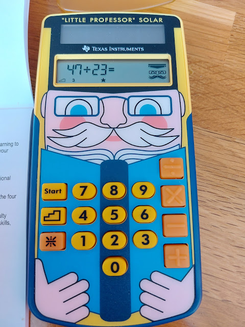
Review: "Little Professor" Solar


If you were a kid during the 1970s and 1980s, like I was, or a parent during that time, the calculator that I am about to review may bring back memories.


Quick Facts


Model:  "Little Professor" Solar (yes, the name is quoted on the calculator)

Company: Texas Instruments 

Years:  2011 - current

Type:  Education

Solar Powered 

Cost:  $ 17.50 US (Texas Instruments Educational Technology Store - 8/21/2022)


Working Our Arithmetic Muscles


The Little Professor Solar is an upgrade of the popular classic Little Professor from 1976.  Unlike the original, the solar version is 100% solar powered without a need for batteries.  


There are two modes:


*  Quiz

*  Arithmetic Tables


Quiz Mode


The Quiz Mode, activated by the [ Start ] key, selects an arithmetic problem to calculate based from one of five levels.  Level 5 is the most difficult, involving mostly two and three digit numbers.  


All the numbers are positive integers.  There is no decimal point, no negative numbers, no fractions.   All division problems divide equally without remainders.


Set the operator by pressing [ + ], [ - ], [ × ], or [ ÷ ].  The stairs button is selects the level, with the mode defaulting to level 1, which is for elementary students.  Levels 2 and higher are great for older students, those who are reviewing arithmetic, and those who want to practice their mental mathematic skills.  Change the level by pressing the key that has a stairs graphic on it (one the left side).  


On minor knock is that there is no contract between font and key on the arithmetic keys, which are bright orange.  I wish these keys would have contrast.  Thankfully, the arithmetic operators are raised so they can be felt.  


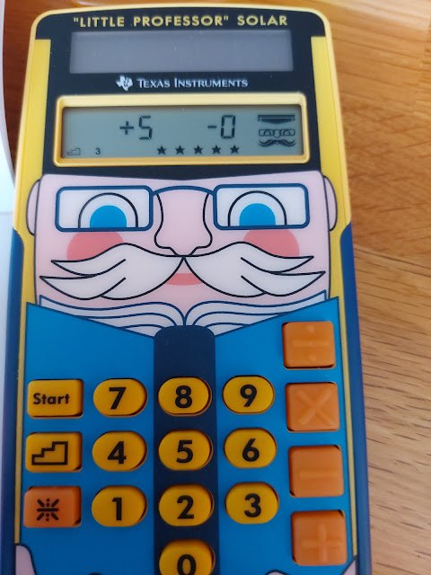
You will have two chances to solve the problem.  It is not timed, so take the time necessary.   After two incorrect answers, the Little Professor shows the correct answer.   After five problems, your score is shown.  The set is on five problems permanently.


The Quiz mode was present on the original Little Professor, but had 10 problems before displaying a score.  


Arithmetic Tables


The second mode is arithmetic drill table, which is activated by pressing the asterisk key  [ * ].  


Again, select an operator and then quickly enter a base within five seconds.  For example, if you want to practice numbers multiplied by 15, enter [ × ] 15.  


Five problems are given.


I don't believe the Arithmetic Tables mode is available on the original Little Professor.  


Final Thoughts


I think the Little Professor can be a compliment to arithmetic flash cards, possibly replace them if you don't want paper goods.  And one thing to remember is that the Little Professor Solar is not just for elementary school students, but can be used for anyone working on their arithmetic skills.  Worth a look and a buy.


There is also an app for the classic (not current) by grebulon for Android:


https://play.google.com/store/apps/details?id=com.grebulon.littleprofessor


Texas Instruments Online Store (United States, Canada, Europe):  https://epsstore.ti.com/OA_HTML/TIibeCCtdMinisites.jsp?ref_url=https%3a%2f%2feducation.ti.com%2fen%2fpurchase%2fpurchase


"Little Professor"  Wikipedia.   Last Edited on July 7, 2022 and accessed on August 21, 2022.  https://en.wikipedia.org/wiki/Little_Professor


Happy calculating,


Eddie 


All original content copyright, © 2011-2022.  Edward Shore.   Unauthorized use and/or unauthorized distribution for commercial purposes without express and written permission from the author is strictly prohibited.  This blog entry may be distributed for noncommercial purposes, provided that full credit is given to the author. 


Saturday, September 10, 2022

DM42: Recursive Fibonacci by Marko Draisma

DM42:  Recursive Fibonacci by Marko Draisma


The programs on today's entry is provided from Marko Draisma and they are provided with permission and a request.  Gratitude to Marko.


DM42 (and Free42/Plus42) Program: FIBO (Marko Draisma)


This recursive program generates the nth Fibonacci number.  FIBO is a recursive program because it calls itself in the program steps.


LBL "FIBO"

LSTO "N"

X>0?

GTO 00

0

RTN

LBL 00

1

RCL "N"

X>Y?

GTO 01

1

RTN

LBL 01

RCL "N"

1

-

XEQ "FIBO"

LSTO "M"

RCL "N"

2

-

XEQ "FIBO"

RCL "M"

+

END


1st Fibonacci number:  1 FIBO returns 1

2nd Fibonacci number:  2 FIBO returns 1

3rd Fibonacci number:  3 FIBO returns 2

4th Fibonacci number:  4 FIBO returns 3

5th Fibonacci number:  5 FIBO returns 5

6th Fibonacci number:  6 FIBO returns 8

7th Fibonacci number:  7 FIBO returns 13


The LSTO Command


This is the local store command.  Local variables are created only for the purpose of the program and are deleted when the program hits either a return command (RTN) or an end command (END).  


Variables created by the LSTO command are named variables.  We cannot create local variables to numeric registers.   There is no storage arithmetic with LSTO.  


LSTO is available for the Swiss Micros DM42, Free42, and the Plus42.


Execution Time of FIBO


The execution time of FIBO depends on how large the entry n. Calculating the 50th Fibonacci number, 12,586,269,025, takes over 12 minutes. Marko provides a fast tail recursion version, as presented next.  


DM42 (and Free42/Plus42) Program: FIBO2 (Marko Draisma)


00 { 80-Byte Prgm }

01▸LBL "FIBO2"

02 FS? 01

03 GTO 01

04 LSTO "N"

05 1

06 LSTO "B"

07 0

08 LSTO "A"

09 SF 01

10 XEQ "FIBO2"

11 RTN

12▸LBL 01

13 RCL "N"

14 X≠0?

15 GTO 02

16 CF 01

17 RCL "A"

18 RTN

19▸LBL 02

20 RCL "A"

21 ENTER

22 RCL+ "B"

23 LSTO "A"

24 X<>Y

25 LSTO "B"

26 RCL "N"

27 1

28 -

29 LSTO "N"

30 XEQ "FIBO2"

31 END


Getting the 50th Fibonacci number with FIBO2 is snap.   


Thanks once again to Marko Draisma.


See you next time,


Eddie 


All original content copyright, © 2011-2022.  Edward Shore.   Unauthorized use and/or unauthorized distribution for commercial purposes without express and written permission from the author is strictly prohibited.  This blog entry may be distributed for noncommercial purposes, provided that full credit is given to the author. 

Friday, September 9, 2022

Casio fx-991EX Classwiz Tips: Tables and Graphs

Casio fx-991EX Classwiz Tips:  Tables and Graphs


This week I am going to show some things that can be done with the Casio fx-991EX Classwiz.  


Believe it or not, the Classwiz can produce graphs of functions.   But not in the way we are used to.  


Generating Tables and Graphs


To generate a table, press [ MENU ], 9: Table.  The Classwiz will always ask for two functions f(x) and g(x).  The function g(x) can be left blank.


You are asked for:

Start:  minimum x value

End:  maximum x value

Step:  change of x


number of steps =  ceiling((End - Start) / Step)


The maximum number of steps for f(x) alone is 45, it gets reduced to 30 if both f(x) and g(x) are used. 


The table of values are displayed.


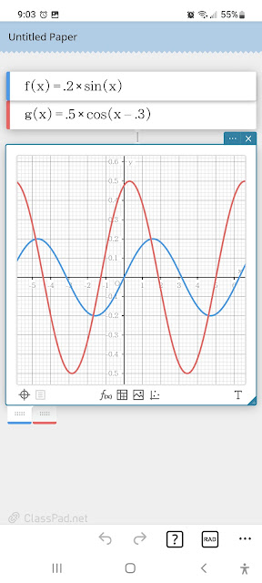
While the table is displayed, you can generate a graph by pressing [SHIFT] (QR).  This has the Classwiz generating a QR code.  You will need a QR reader, which you can use the Casio EDU app to read the code.


Once the QR code fits into the camera, you are given a link.  Below are examples of graphs:


I hope this week has been helpful in highlighting some of the features of the Casio Classwiz.   For the students in school, I wish you a happy and successful school year.


The next blog post will be on September 15, 2022.   Also, I am going to talk about HHC 2022 in Nashville.  


Eddie


All original content copyright, © 2011-2022.  Edward Shore.   Unauthorized use and/or unauthorized distribution for commercial purposes without express and written permission from the author is strictly prohibited.  This blog entry may be distributed for noncommercial purposes, provided that full credit is given to the author. 


Thursday, September 8, 2022

Casio fx-991EX Classwiz Tips: Normal Distribution

Casio fx-991EX Classwiz Tips:  Normal Distribution


This week I am going to show some things that can be done with the Casio fx-991EX Classwiz.  


The Normal Distribution 


The Classwiz's Distribution mode has calculations for the following probability distributions:


1.  Normal, f(x) = exp(-1/2 * ((x - μ) / σ)^2 ) / (σ * √(2 * π))

2.  Binomial

3.  Poisson


This is Mode 7.


Normal CD - Finding the Area


[ MENU ], 7: Distribution, 2: Normal CD


The CDF function calculates the area (probability) between two limits.   The lower and upper tail areas require the limits to be -∞ and +∞, respectively.  However, the Classwiz does not provide values for -∞ and +∞.  For the best estimate, I suggest using -7 and 7 are the limits.  The calculator calculates the probability from -7 to 7 to be 1.


Example:

(For all the examples, the standard values μ = 0, σ = 1)


Lower tail area to x = 3:  lower limit = -7, upper limit = 3; area:  0.9986501019


Lower limit = -2, upper limit = 2; area:  0.954499736


Upper tail from x = -1:  lower limit = 1, upper limit = 7; area:  0.1586552539


Inverse CD


[ MENU ], 7: Distribution, 3: Inverse Normal


This calculation gets the point value for a lower tail distribution (-∞ to x).


Example:

(For all the examples, the standard values μ = 0, σ = 1)


Area = 0.5; xInv:  0


Area = 0.6; xInv: 0.2533470931


Area = 0.7; xInv: 0.5244004382


Eddie


All original content copyright, © 2011-2022.  Edward Shore.   Unauthorized use and/or unauthorized distribution for commercial purposes without express and written permission from the author is strictly prohibited.  This blog entry may be distributed for noncommercial purposes, provided that full credit is given to the author. 


Wednesday, September 7, 2022

Casio fx-991EX Classwiz Tips: Solve for Any Variable

Casio fx-991EX Classwiz Tips:  Solve for Any Variable


This week I am going to show some things that can be done with the Casio fx-991EX Classwiz.  


Solving For Any Variable


The Casio Classwiz can solve equations in the main (Calculate) mode in the following formats:


Equation, i.e.  A + 2x = y^3

And Expression Equal to Zero, i.e. 2x^4 - 18  (the equal to zero is implied)


Pressing [SHIFT] [CALC] (SOLVE) allows us to enter values for all but one variable to solve for.   Enter values with the equals [ = ] key.  


When you select the variable to solve for, press the [ = ] key without entering a number.


Caution:  When you are entering equations, don't use the white [ = ] key.  To enter the = character, press [ALPHA] [ CALC ].


The L-R indicator tells the the accuracy of the solution.  We want L-R = 0.


Example:


2x^2 + 3y^3 = A


Keystrokes:  2 [ x ] [ x^2 ] [ + ] 3 [ALPHA] (Y) [SHIFT] (x^3) [ALPHA] (=) [ALPHA] (A)

[SHIFT] (SOLVE)


Inputs:  x = 8, y = 2, solve for A.   A = 152, L-R = 0


Inputs:  x = 6, A = 79, solve for y.  y = 1.326352406, L-R = 0


Inputs: y = 3.5, A = 105, solve for x.  Cannot Solve   (x has a complex number solution)


Eddie


All original content copyright, © 2011-2022.  Edward Shore.   Unauthorized use and/or unauthorized distribution for commercial purposes without express and written permission from the author is strictly prohibited.  This blog entry may be distributed for noncommercial purposes, provided that full credit is given to the author. 


Tuesday, September 6, 2022

Casio fx-991EX Classwiz Tips: Solving Inequalities

Casio fx-991EX Classwiz Tips:  Solving Inequalities


This week I am going to show some things that can be done with the Casio fx-991EX Classwiz.  


Solving Inequalities


Did you know that the Casio Classwiz can solve inequalities in the forms:


p(x) > 0

p(x) <0

p(x) ≥ 0

p(x) ≤ 0


where p(x) is a polynomial of degree 2 to 4.   The lead coefficient is nonzero.


To get there:  [MENU], [ ° ' " ] (B).


Each inequality and answers are displayed in textbook format.


Examples:


-4x^2 + 8x - 1 < 0

Result:  x < (2 - √3)/2, (2 + √3)/2 < x


-4x^2 + 8x - 1 > 0

Result:  (2 - √3)/2 < x < (2 + √3)/2


3x^4 + 0x^3 - 8x^2 - 6x + 5 ≥ 0

Result:  x≤0.5149391226, 1.8065398762≤x


Eddie


All original content copyright, © 2011-2022.  Edward Shore.   Unauthorized use and/or unauthorized distribution for commercial purposes without express and written permission from the author is strictly prohibited.  This blog entry may be distributed for noncommercial purposes, provided that full credit is given to the author. 


Numworks: Allowing Repeated Calculations in Python

Numworks: Allowing Repeated Calculations in Python Introduction Say we want the user to repeat a calculation or a routine for as lo...