Spotlight: TI-32 Solar from 1988

Spotlight: TI-32 Solar from 1988

Today’s spotlight is on a standard scientific calculator from Texas Instruments… with a twist. First, let’s start with the quick facts.

Quick Facts

Model: TI-32 Solar

Company: Texas Instruments

Timeline: 1988 (possibly 1989?), this model was very short lived

Type: Scientific

Memory: 1 memory register

Power: Solar

Screen: 10 digits

The TI-32 Solar was a scientific calculator that was sold briefly by Texas Instruments in the last 1980s. The function set is a combination of the TI-30 Solar and the original one line TI-34:

* trigonometry, decimal/dms conversion, rectangular/polar conversions

* logarithms, anti-logarithms (10^x, e^x), powers

* one variable statistics (mean, deviation, sums)

* binary/decimal/hexadecimal conversion (and just conversions, strangely no octal)

* 3-decimal random number generator (RND)

* percent function

The Polar/Rectangular conversions use the [ a ] and [ b ] keys. [ a ] is for x and r, while [ b ] is for y and Θ.

The statistics mode is one-variable only. Though I am not a fan of the STAT mode being the alternative function of the [ C ] key, thankfully, the stat mode works.

What truly sets the TI-32 Solar apart are two things:

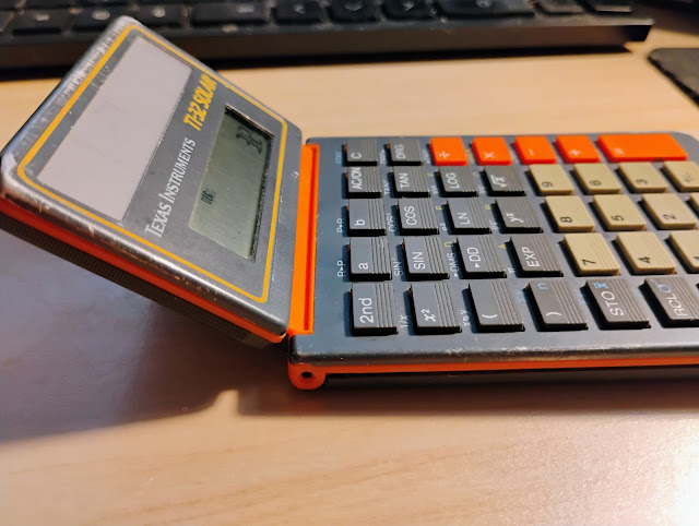
(1) The orange trim and keys on a dark gray keyboard. This is a very rare color scheme, especially orange until Texas Instruments started to release the TI-30XIIS and the TI-84 Plus CE in various colors.

(2) The screen tilts. The screen is a set on a hinge that allows the user to tilt the screen to different angles, which allows for more ergonomic operation. To put the calculator away, tilt the screen to be aligned with the keyboard and use the slide case. I think this is a really neat idea. The tilt mechanism seems to hold out well for a nearly 40 year old calculator.

Source

Woerner, Joerg. “Texas Instruments TI-32 SOLAR” Datamath Calculator Museum. September 20, 2002. Accessed July 7, 2025. http://www.datamath.org/Sci/Modern/TI-32Solar.htm

Eddie

 All original content copyright, © 2011-2025. Edward Shore. Unauthorized use and/or unauthorized distribution for commercial purposes without express and written permission from the author is strictly prohibited. This blog entry may be distributed for noncommercial purposes, provided that full credit is given to the author.

All posts are 100% generated by human effort.  The author does not use AI engines and never will.

HP 71B and HP Prime Python: Gaussian Quadrature

HP 71B and HP Prime Python: Gaussian Quadrature

A Very Brief Introduction

This is a top-level overview of the Gaussian Quadrature method. For more details, please check out the Sources section.

The design of GQ is to calculate:

∫( f(x) dx, -1, 1) ≈ Σ( wi * f(xi), i = 1, n)

Where do xi and wi come from?

* The xi values come from find the roots of the polynomials P’(x)= 0

* Pn’(x) are the derivatives of the Legendre polynomials Pn(x)

* After getting the roots, xi, the weights, w are calculated by the formula:

wi = 2 / ((1 -xi)^2 * Pn’(xi)^2)

Weights and Points of orders 3 and 5:

Among 3 points:

Roots (x) come from the derivative of the Legendre polynomial of the 3^rd order.

Pn’(x) = 3/2 * (5*x^2 – 1)

Point xi	Weight wi
-√(3/5) ≈ -0.7745 9669 2 = -√0.6	5/9
0	8/9
√(3/5) ≈ 0.7745 9669 2 = √0.6	5/9

Among 5 points:

Roots (x) come from the derivative of the Legendre polynomial of the 5^th order.

Pn’(x) = 15/8 * (21*x^4 – 14*x^2 + 1)

Point xi	Weight wi
-0.90617 98459	0.23692 68851
-0.53846 93101	0.47862 86705
0	128/225 ≈ 0.56888 88889
0.53846 93101	0.47862 86705
0.90617 98459	0.23692 68851

We can fit any interval [a, b] by this conversion:

∫( f(x) dx, a, b) = (b – a) / 2 * ∫( f( (b – a) / 2* x + (b + a) / 2 dx, -1, 1)

= (b – a) / 2 * Σ( wi * f( (b – a) / 2 * xi + (b + a) / 2 ), i = 1, n)

However, the programs on this blog entry will focus on the basic version of the Gaussian Quadrature.

The Code

The following code works with the following integrals:

∫( f(x) dx, -1, 1) ≈ Σ( wi * f(xi), i = 1, n)

HP 71B Basic

HP 71B: GQ3 (Gaussian Quadrature – 3 Point: Integrals from -1 to 1)

10 DEF FNF(X) = insert function of X here

15 S = 0

20 RADIANS

25 FOR I = 1 TO 3

30 READ X, W

31 DATA -SQR(0.6),5/9

32 DATA 0,8/9

33 DATA SQR(0.6),5/9

40 S = S + W * FNF(X)

55 NEXT I

50 DISP “ INTEGRAL= ”; S

HP 71B: GQ5 (Gaussian Quadrature – 5 Point: Integrals from -1 to 1)

10 DEF FNF(X) = insert function of X here

15 S = 0

20 RADIANS

25 FOR I = 1 TO 5

30 READ X, W

31 DATA -.9061798459, .2369268851

32 DATA -.5384693101, .4786286705

33 DATA 0, 128/255

34 DATA .5384693101, .4786286705

35 DATA .9061798459, .2369268851

40 S = S + W * FNF(X)

45 NEXT I

50 DISP “ INTEGRAL= ”; S

Integral Test: ∫( f(x) dx, -1, 1) ≈ Σ( wi * f(xi), i = 1, n)

Function f(x)	Actual (approx)	Gaussian 3 point (GQ3)	Gaussian 5 point (GQ5)
(x-3)*(x+4)*(x-5)	352/3 ≈ 117.333333333	117.333333333	117.333333334
-x^2 + 9*x + 10	58/3 ≈ 19.33333333	19.3333333334	19.3333333333
1.5 * cos(x)	2.524412954	2.52450532159	2.52441295561
exp(-x)	2.350402387	2.35033692868	2.35040238646
exp(sin(x))	2.283194521	2.28303911433	2.28319665353
sin(x)	0	0	0
1/(x - 2)	-1.09861228867	-1.09803921569	-1.09860924181

HP Prime Python App

HP Prime Python: gq3.py

# Gaussian Quadrature 3 point

from math import *

def f(x):

  # insert Function here

  return 1/(x-2)

s=0

x=[-sqrt(0.6),0,sqrt(0.6)]

w=[5/9,8/9,5/9]

for i in range(3):

  s=s+w[i]*f(x[i])

print("Integral: ",s)

HP Prime Python: gq5.py

# Gaussian Quadrature 5 point

from math import *

def f(x):

  # insert Function here

  return sin(x)

s=0

x=[0,-.5384693101056831,.5384693101056831,-.9061798459386640, .9061798459386640]

w=[.5688888888889,.4786286704993665,.4786286704993665,.2369268850561891,.2369268850561891]

for i in range(5):

  s=s+w[i]*f(x[i])

print("Integral: ",s)

Function f(x)	Actual (approx)	Gaussian 3 point (GQ3)	Gaussian 5 point (GQ5)
(x-3)*(x+4)*(x-5)	352/3 ≈ 117.333333333	117.333333333	117.333333333
-x^2 + 9*x + 10	58/3 ≈ 19.33333333	19.3333333333	19.3333333334
1.5 * cos(x)	2.524412954	2.52450532159038	2.52441295561081
exp(-x)	2.350402387	2.35033692868001	2.35040238646284
exp(sin(x))	2.283194521	2.2830391143268	2.28319665352905
sin(x)	0	0.0	0.0
1/(x - 2)	-1.09861228867	-1.09803921568627	-1.09860924181248

Sources

Kamermans, Mike “Pomax”. “Gaussian Quadrature Weights and Abscissae” https://pomax.github.io/bezierinfo/legendre-gauss.html 2011. Retrieved January 19, 2025.

Wikipedia. “Gauss-Legendre quadrature” https://en.wikipedia.org/wiki/Gauss%E2%80%93Legendre_quadrature Last edited January 19, 2025. Retrieved January 19, 2025.

Wikipedia. “Legendre Polynomials” https://en.wikipedia.org/wiki/Legendre_polynomials Last edited December 4, 2024. Retrieved January 19, 2025.

When it comes to evaluating integrals numerically, is Gaussian Quadrature better than Simpson’s Method?

Eddie

 All original content copyright, © 2011-2025. Edward Shore. Unauthorized use and/or unauthorized distribution for commercial purposes without express and written permission from the author is strictly prohibited. This blog entry may be distributed for noncommercial purposes, provided that full credit is given to the author.

The content on this blog is 100% generated by humans. The author does not use AI engines and never will.

fx-3900PV Programs: Finance Factors

fx-3900PV Programs: Finance Factors

I’m revisiting the fx-3900Pv, which seems to be a hit. The last set of programs from May 3 of this year: https://edspi31415.blogspot.com/2025/05/casio-fx-3900pv-linear-system-poisson.html

Remember: When using the ENT (enter/input) command, we must enter a valid number and then the next step. The number that precedes ENT is not counted as a step and is not recorded.

Example: x + 9

In LRN (learn) mode (Mode EXP):

ENT (enter any number)

+

9

=

Casio fx-3900Pv: Simple Interest

maturity amount = principal amount * (1 + 0.01 * I%) * N ÷ 360

interest accrued = maturity amount – principal amount

I% = annual interest rate

N = number of days

The Act/360 method is used.

Code (23 steps):

ENT # enter principal amount (PV)

Kin 1

×

(

1

+

.

0

1

×

ENT # enter interest rate

×

ENT # enter number of days

÷

3

6

0

)

=

HLT # pause, display maturity amount

-

Kout 1

= # display interest accrued, end program

Example 1:

Inputs:

Principal Amount: 1,000.00

Rate: 5%

Number of Days: 30

Output (rounded to 2 decimal places)

Maturity Amount: 1,004.17

Interest Accrued: 4.17

Example 2:

Inputs:

Principal Amount: 360.00

Rate: 8%

Number of Days: 90

Output (rounded to 2 decimal places)

Maturity Amount: 367.20

Interest Accrued: 7.20

Casio fx-3900Pv: Compound Interest Factor with Compounding Periods

The following program calculates the compound interest factor:

factor = (1 + I% ÷ PYR) ^ (YRS × PVR)

where

I% = annual interest rate

PYR = payments per year (compounding periods)

YRS = number of years (N)

The factor is used in simple compound interest problems:

FV = PV × factor

where:

FV = future value

PV = present value

Code (19 steps):

(

1

+

.

0

1

×

ENT # enter interest rate

÷

ENT # enter payments per year

Kin 1

)

x^y

(

ENT # enter number of years

×

Kout 1

)

=

Example:

Find the compound interest interest factor for: I% = 5%, 12 payments a year, 4 years

Factor: 1.220895351

If an investor expects a $5,000.00 payoff, what should the investor pay?

PV = FV ÷ X

Keys: (with the answer from program displayed: [ 1/x ] [ × ] 5000 [ = ])

PV (rounded): 4,0953.36

Casio fx-3900Pv: Loan Annuity Factor

The following program calculates the loan annuity factor:

factor = ( ( 1 - ( 1 + I% ÷ PYR ) ^ (-YRS × PYR) ) ÷ ( I% ÷ PYR )

where

I% = annual interest rate

PYR = payments per year (compounding periods)

YRS = number of years (N)

The factor is used in loan problems without balloon payments, and assume that the payments occur at the end of each period (ordinary annuity):

PV = PMT × factor

where:

PV = present value

PMT = periodical payments

Code (30 steps):

ENT # enter interest rate

÷

ENT # enter payments per year

Kin 2

×

.

0

1

=

Kin 1 # K1 = I% ÷ PYR

ENT # enter number of years

×

Kout 2

=

Kin 2 # K2 = YRS × PYR = N

(

1

-

(

1

+

Kout 1

)

x^y

Kout 2

+/-

)

÷

Kout 1

=

Example:

A student buys a car at $35,619 (after taxes and fees). The student gets a six year loan at 5.7% and pays at the end of each month. What is the payment?

PMT = PV ÷ factor

where PV = 35619, I% = 5.7, PYR = 12 (monthly payments), YRS = 6

Running the program with inputs 5.7, 12, 6: 60.85819003

Payment: [ 1/x ] [ × ] 35619 [ = ]: 585.28 (rounded)

Casio fx-3900Pv: Sinking Fund Factor (Savings Account)

The following program calculates the sinking factor (used for savings accounts):

factor = ( (1 + I% ÷ PYR) ^ (YRS × PYR) – 1 ) ÷ (I% ÷ PYR)

The factor is used in determining the future value of savings plans with regular deposits made at the end of each period:

FV = PMT × factor

Code (29 steps):

ENT # enter interest rate

÷

ENT # enter payments per year

Kin 2

×

.

0

1

=

Kin 1 # K1 = I% ÷ PYR

ENT # enter the number years

×

Kout 2

=

Kin 2 # K2 = YRS × PYR

(

(

1

+

Kout 1

)

x^y

Kout 2

-

1

)

÷

Kout 1

=

Example:

A child’s parents opens up an account on the child’s first birthday. The parents contribute $200.00 per month for the next 18 years. The account pays a fixed rate of 3% per month. What is the value of the fund when the child turns 18?

Note: The account is opened on the child’s first birthday, hence 17 years pass.

FV = PMT × factor

where PMT = 100, I% = 3, PYR = 12, YRS = 17

Running the program with inputs 3, 12, 17: 265.69267

Future Value: [ × ] 200 [ = ]: 53,138.54 (rounded)

Until next time, stay safe and sane,

Eddie

All original content copyright, © 2011-2025. Edward Shore. Unauthorized use and/or unauthorized distribution for commercial purposes without express and written permission from the author is strictly prohibited. This blog entry may be distributed for noncommercial purposes, provided that full credit is given to the author.

The content on this blog is 100% generated by humans. The author does not use AI engines and never will.