AOS Calculators: Duplicating a Value Without Retyping It

AOS Calculators: Duplicating a Value Without Retyping It

Note: The following applies to scientific classic calculators who operate under the algebraic operating system (AOS) (that is what Texas Instrument’s calls it). I tested this procedure with the following calculators: TI-30X ECO, HP 10bII+ (Algebraic mode), and Casio fx-260 Solar.

Introduction: Going Back to 1976

Imagine it is 1976 and you have have an SR-56 from Texas Instruments. Here is what an SR-56 looks like: http://www.datamath.org/Sci/WEDGE/ZOOM_SR-56.htm

You are tasked to calculate 1.401103287^1.401103287 and do not want to write the number twice. According to page 53 of the SR-56 manual, one approach is to key in:

1.401103287 [ y^x ] [ CE ] [ = ]

Result: 1.604057054

For that particular calculator, SR-56, pressing [ CE ] once stores the number in the display as the second operand allowing the value to duplicated without having to retype the number.

If we tried that on a modern TI-30Xa/TI-30 ECO RS, the display would clear to zero instead of showed the previous number.

However, there are a few tricks we can employ to achieve the similar result.

Trick 1: Pressing the Reciprocal Key Twice

As long as the number in the display is nonzero, pressing [ 1/x ] [ 1/x ] registers the number in the display for as a second operand. In calculators operating in AOS, executing one-argument functions only operate and effect the number in the display only.

Pressing [ 1/x ] takes the reciprocal of the number and registers the number in the display. Pressing [ 1/x ] again returns the number.

**The keystrokes omits any [ 2^nd ] or [ SHIFT ] keys.

Example 1:

Expression: x * log x

Keystrokes: x [ × ] [ 1/x ] [ 1/x ] [ LOG ] [ = ]

5.8 * log 5.8

Keystrokes: 5.8 [ × ] [ 1/x ] [ 1/x ] [ LOG ] [ = ]

Result: 4.427882363

Example 2:

Expression: x^x

Keystrokes: x [ y^x ] [ 1/x ] [ 1/x ] [ = ]

3.088 ^ 3.088

Keystrokes: 3.088 [ y^x ] [ 1/x ] [ 1/x ] [ = ]

Result: 32.51797379

Example 3:

Expression: x * sin x

Keystrokes: x [ × ] [ 1/x ] [ 1/x ] [ SIN ] [ = ]

50° * sin 50°

Keystrokes: ([DRG] to DEG/[ MODE ] (DEG))

50 [ × ] [ 1/x ] [ 1/x ] [ SIN ] [ = ]

Result: 38.30222216

4^4 + 1 / (3^3)

Keystrokes:

4 [ y^x ] [ 1/x ] [ 1/x ] [ + ]

[ ( ] 3 [ y^x ] [ 1/x ] [ 1/x ] [ ) ] [ 1/x ] [ = ]

Result: 256.037037

If the calculator has a cube function (x^3), we can execute this keystroke:

4 [ y^x ] [ 1/x ] [ 1/x ] [ + ]

[ ( ] 3 [ x^3 ] [ ) ] [ 1/x ] [ = ]

Trick 2: Inverse Function Trick

This trick extends the reciprocal trick to include a function that acts on two (and theoretically more) “reversible” functions. This trick applies to the expressions with the following format:

f(x) OP g(x)

f(x)	f^-1(x)	f(x)	f^-1(x)	f(x)	f^-1(x)
SIN	SIN^-1	e^x	LN	X^3	∛
COS	COS^-1	LN	e^x	∛	X^3
TAN	TAN^-1	10^x	LOG	Hyperbolic	Inverse Hyperbolic
SIN^-1	SIN	LOG	10^x	Inverse Hyperbolic	Hyperbolic
COS^-1	COS	X^2	√
TAN^-1	TAN	√	X^2

OP covers the arithmetic operations: [ + ], [ - ], [ × ], [ ÷ ], [ y^x ], and [ y^(1/x) ]

The general keystroke sequence is: x [ f(x) ] [ OP ] [ f^-1(x) ] [ g(x) ] [ = ]

Let’s illustrate this with a few examples. Assume the calculator is in degrees mode.

Example 1:

sin 40° * cos 40°

f(x) = sin x, f^-1(x) = sin^-1 x, g(x) = cos x

Keystrokes: 40 [ SIN ] [ × ] [ SIN^-1 ] [ COS ] [ = ]

Result: 0.492403877

Example 2:

tan 32° * sin 32°

f(x) = tan x, f^-1(x) = tan^-1 x, g(x) = sin x

Keystrokes: 32 [ TAN ] [ × ] [ TAN^-1 ] [ SIN ] [ = ]

Result: 0.331130307

Example 3:

log 881 * ln 881

f(x) = log x, f^-1(x) = 10^x, g(x) = ln x

Keystrokes: 881 [ LOG ] [ × ] [ 10^x ] [ LN ] [ = ]

Result: 19.97005314

Example 4:

e^3.5 / √3.5

f(x) = e^x, f^-1(x) = ln x, g(x) = √x

Keystrokes: 3.5 [ e^x ] [ ÷ ] [ LN ] [ √ ] [ = ]

Result: 17.70095363

Example 5:

√4.555 + e^4.555

f(x) = √x, f^-1(x) = x^2, g(x) = e^x

Keystrokes: 4.555 [ √ ] [ + ] [ x^2 ] [ e^x ] [ = ]

Result: 97.24099983

The inverse function “recovers and registers” the original x. It’s kind of simulating the LAST x feature on RPN calculators.

Sources

Datamath. “Texas Instruments SR-56“ December 5, 2001. http://www.datamath.org/Sci/WEDGE/SR-56.htm

Texas Instruments. Programmable Slid-Rule Calculator SR-56: Owner’s Manual. Dallas, TX. 1976

Eddie

All original content copyright, © 2011-2025. Edward Shore. Unauthorized use and/or unauthorized distribution for commercial purposes without express and written permission from the author is strictly prohibited. This blog entry may be distributed for noncommercial purposes, provided that full credit is given to the author.

All posts are 100% generated by human effort.  The author does not use AI engines and never will.

TI-30Xa Algorithms: Linear Regression

 TI-30Xa Algorithms: Linear Regression

Welcome to the March 2024 installment of TI-30Xa Algorithms.

Linear Regression with a TI-30Xa?

Today’s task is to fit bi-variate data to the line:

y = m * x + b

with the TI-30Xa. What? This calculator does not have a linear regression mode. Yes, with it is possible. We are going to use the technique shown in by the TI-36 Solar Guidebook from 1985 (see Source below). The TI-36 Solar was part of Texas Instruments’ line in the late 1980s and the early 1990s.

You can read my review on the TI-36 Solar from September 26, 2020 here:

https://edspi31415.blogspot.com/2020/09/retro-review-ti-36-solar.html

Where the TI-36 Solar only had one memory register, the TI-30Xa has three memory registers, and they are going to come in handy here.

Procedure

Caution: Be sure the calculator is on the entire time. Turning off the calculator will clear out statistics mode.

1. Enter the y data. Store the mean (y-bar) into memory register 2. Store the population deviation (σy) into memory register 3.

Keystrokes:

Mean of y-data: [ 2^nd ] [ x^2 ] {x-bar} [ STO ] [ 2 ]

Population of y-data: [ 2^nd ] [ ÷ ] { σxn } [ STO ] [ 3 ]

2. Clear the stat registers and enter the x data. As we are entering the x data, use memory register 1 to calculate Σxy.

Keystrokes:

Clear Stat Registers: [ 2^nd ] [ 7 ] {CSR}

1^st Point:

x1 [ × ] y1 [ = ] [ STO ] [ 1 ]

x1 [ Σ+ ]

Every point there after:

x_i [ × ] y_i [ = ] [ 2^nd ] [ RCL ] {SUM} [ 1 ]

x_i [ Σ+ ]

3. Calculate the slope, and replace Σxy with the slope.

m = ( y-bar * Σx – Σxy) / ( x-bar * Σx - Σx^2)

Keystrokes:

[ ( ] [ RCL ] [ 2 ] [ × ] [ 2^nd ] [ ( ] [ - ] [ RCL ] [ 1 ] [ ) ]

[ ÷ ] [ ( ] [ 2^nd ] [ x^2 ] [ × ] [ 2^nd ] [ ( ] [ - ] [ 2^nd ] [ ) ] [ = ] [ STO ] [ 1 ]

4. Calculate the y-intercept, replace y-bar with the y-intercept.

b = -m * x-bar + y-bar

Keystrokes:

[ RCL ] [ 1 ] [ +/- ] [ × ] [ 2^nd ] [ x^2 ] [ + ] [ RCL ] [ 2 ] [ = ] [ STO ] [ 2 ]

5. Calculate the correlation. If the correlation is close to -1 or +1, the linear fit will be excellent.

r = m * σx / σy

Keystrokes:

[ RCL ] [ 1 ] [ × ] [ 2^nd ] [ ÷ ] [ ÷ ] [ RCL ] [ 3 ] [ = ]

6. Use slope (m) and intercept (b) to predict x and y values:

y’ = m * x0 + b

Keystrokes: [ RCL ] [ 1 ] [ × ] x0 [ + ] [ RCL ] [ 2 ] [ = ]

x’ = (y0 – b) / m

Keystrokes: [ ( ] y0 [ - ] [ RCL ] [ 2 ] [ ) ] [ ÷ ] [ RCL ] [ 1 ] [ = ]

Key Map

[ RCL ] [ 1 ]: first Σxy, then m

[ RCL ] [ 2 ]: first y-bar, then b

[ RCL ] [ 3 ]: σy

[ 2^nd ] [ x^2 ]: x-bar

[ 2^nd ] [ ÷ ]: σxn

Example

Fit a line to the data:

X	Y
12	100
13	98.7
14	97.1
16	94.9
18	92.6
20	90

1. Enter the y data. Store the mean (y-bar) into memory register 2. Store the population deviation (σy) into memory register 3.

100 [ Σ+ ]

98.7 [ Σ+ ]

97.1 [ Σ+ ]

94.9 [ Σ+ ]

92.6 [ Σ+ ]

90 [ Σ+ ] (display n = 6)

Mean of y-data: [ 2^nd ] [ x^2 ] [ STO ] [ 2 ] (y-bar = 95.55)

Population of y-data: [ 2^nd ] [ ÷ ] [ STO ] [ 3 ] (σy = 3.465424457)

2. Clear the stat registers and enter the x data. As we are entering the x data, use memory register 1 to calculate Σxy.

Keystrokes:

Clear Stat Registers: [ 2^nd ] [ 7 ] {CSR}

12 [ × ] 100 [ = ] [ STO ] [ 1 ]

12 [ Σ+ ]

13 [ × ] 98.7 [ = ] [ 2^nd ] [ RCL ] [ 1 ] (SUM 1)

13 [ Σ+ ]

14 [ × ] 97.1 [ = ] [ 2^nd ] [ RCL ] [ 1 ] (SUM 1)

14 [ Σ+ ]

16 [ × ] 94.9 [ = ] [ 2^nd ] [ RCL ] [ 1 ] (SUM 1)

16 [ Σ+ ]

18 [ × ] 92.6 [ = ] [ 2^nd ] [ RCL ] [ 1 ] (SUM 1)

18 [ Σ+ ]

20 [ × ] 90 [ = ] [ 2^nd ] [ RCL ] [ 1 ] (SUM 1)

20 [ Σ+ ]

RCL 1: Σxy = 8827.7

[ 2^nd ] [ x^2 ]: x-bar = 15.5

3. Calculate the slope, and replace Σxy with the slope.

[ ( ] [ RCL ] [ 2 ] [ × ] [ 2^nd ] [ ( ] [ - ] [ RCL ] [ 1 ] [ ) ]

[ ÷ ] [ ( ] [ 2^nd ] [ x^2 ] [ × ] [ 2^nd ] [ ( ] [ - ] [ 2^nd ] [ ) ] [ = ] [ STO ] [ 1 ]

Slope: m = -1.230526316

4. Calculate the y-intercept, replace y-bar with the y-intercept.

[ RCL ] [ 1 ] [ +/- ] [ × ] [ 2^nd ] [ x^2 ] [ + ] [ RCL ] [ 2 ] [ = ] [ STO ] [ 2 ]

Intercept: b = 114.6231579

5. Calculate the correlation.

[ RCL ] [ 1 ] [ × ] [ 2^nd ] [ ÷ ] [ ÷ ] [ RCL ] [ 3 ] [ = ]

Correlation: r = -0.999092386

The line is:

y = -1.230526316 * x + 114.6231579

6. Predict values.

If x = 15, predict the y value (y’):

[ RCL ] [ 1 ] [ × ] x0 [ + ] [ RCL ] [ 2 ] [ = ]

y’ = 96.16526316

If y = 95, predict the x value (x’):

[ ( ] y0 [ - ] [ RCL ] [ 2 ] [ ) ] [ ÷ ] [ RCL ] [ 1 ] [ = ]

x’ = 15.94696322

Source

Alley, Chris M., Brenda M. Cornitius, et al. TI-36 Solar Guidebook Texas Instruments Incorporated. Dallas, TX. 1985, 1986, 1987. pp. 4.6 – 4.13

Eddie

All original content copyright, © 2011-2024. Edward Shore. Unauthorized use and/or unauthorized distribution for commercial purposes without express and written permission from the author is strictly prohibited. This blog entry may be distributed for noncommercial purposes, provided that full credit is given to the author.

HP 32SII: Glide Slope Calculations (and Memory Management)

HP 32SII:  Glide Slope Calculations (and Memory Management)

Note:   These programs should work on the Swiss Micros DM32.  

Introduction

The following program calculates the forces and angle for a flight of a glider, an aircraft without a engine:

*  Weight

*  Lift Force

*  Drag Force

SI units are used.

With inputs glide distance (G), height (H), and mass (M):

Angle:  A = arcsin(H ÷ G)

Weight:  W = M × 9.80665

Lift:  L = W × sin A

Drag:  D = W × cos A

The program uses the polar-to-rectangular conversion to calculate lift and drag. 

HP 32SII Programs:  Glide Slope Calculations

Code 1:

G01  LBL G

G02  DEG

G03  INPUT G

G04  INPUT H

G05  INPUT M

G06  R↓

G07  x<>y

G08  ÷

G09  ASIN

G10  STO A

G11  VIEW A

G12  R↑

G13  9.80665

G14  ×

G15  STO W

G16  VIEW W

G17  θ,r→y,x

G18  STO L

G19  VIEW L

G20  x<>y

G21  STO D

G22  VIEW D

G23  RTN

Bytes:  42.5

Checksum:  4717

Notes:

*  This version has prompts and view commands to guide the user.  We don't have to preload registers as the INPUT commands guide us.

*  All inputs and outputs are stored to variables.   7 variables are used, which will require 56 bytes.  On the HP 32SII, each variable that contains non-zero values takes 8 bytes of memory.  If you want to make the variables local, insert a CLVARS command for G23 and line G24 becomes RTN.

Variables:

Input:

G = Glide Distance.  The distance that glider climbs to it's peak.   Think of the hypotenuse of a right triangle.   Distance is in meters.  

H = Height.  The height that the glider reaches.  Distance is in meters.

M = Mass.  Mass of the glider in kilograms.

Output:

A = Angle.  Angle of the of glider's flight in degrees. 

W = Weight.  Weight of the glider, which is Newtons.

L = Lift force of the glider, in Newtons.

D = Drag force of the glider, in Newtons.

Code 2:

Code 2 is a shorter code which does not store anything into variables.   The program starts with G (glide distance), H (height), and M (mass) on the stack.  

L01   LBL L

L02   DEG

L03   R↓

L04   x<>y

L05   ÷

L06   ASIN

L07   STOP  (display A)

L08   R↑

L09   9.80665

L10   ×

L11   STOP  (display W)

L12   θ,r→y,x

L13   RTN    (L is on the x stack, D is on the y stack)

Bytes:  27.5 bytes

Checksum:  6446

Examples

Example 1:

Glider distance:  G = 178 m

Height:  H = 23 m

Mass of the glider:  M = 55 kg

Output:

Angle:  A ≈ 7.4241°

Weight:  W ≈ 539.3658 N

Lift:  L ≈ 534.8441 N

Drag:  D ≈ 69.6933 N

Example 2: 

Glider distance:  G = 200 m

Height:  H = 30 m

Mass of the glider:  M = 39 kg

Output:

Angle:  A ≈ 8.6269°

Weight:  W ≈ 382.4594 N

Lift:  L ≈ 378.1322 N

Drag:  D ≈ 57.3689 N

Source

National Museum of the United States Air Force.  "Mathematics of Flight:  Glide Slope II"  September 2020.  Retrieved August 2023.   

https://www.nationalmuseum.af.mil/Portals/7/Mathematics%20of%20Flight%20Glide%20Slope%20II.pdf

Eddie 

All original content copyright, © 2011-2023.  Edward Shore.   Unauthorized use and/or unauthorized distribution for commercial purposes without express and written permission from the author is strictly prohibited.  This blog entry may be distributed for noncommercial purposes, provided that full credit is given to the author. 

Retro Review: Sears Electronic Slide Rule

Retro Review: Sears Electronic Slide Rule

Quick Facts

Model: Electric Slide Rule,  801.58771

Company: Sears

Production Years:  1974 - mid 1970s

Power:  Battery, originally AA chargeable NiCad*

Type:  Scientific

Operating System:  Chain

Memory Registers:  1

Display:  One line:  8 digits, 2 lights:  one for overflow (error), one for negative numbers

Same Key Set as:   Rockwell 61R

*  I purchased this calculator at the Pasadena City College Swap Meet on July 2, 2023.  The calculator is in great condition, along with a great leather case and instruction manual.   The calculator was re-configured to run on 4 regular AA batteries, to that I'm very grateful.

Keyboard and Scientific Functions 

Most of the functions available are shifted functions.  The equals key is in an usual place, on the 2nd row from the top, above the arithmetic keys.  Access the shifted functions (written in white) by pressing the black key [ f ]. 

Scientific Functions Available:

Logarithm:  ln, log, e^x, 10^x

Roots and Powers:  √x, x^y, 1/x

Trigonometry:  sin, cos, tan, arc (inverse)

Memory Functions:  m+, m-, m+x^2  (add the square of a display to memory) x←m (recall), x→m (store), x←→m (exchange with memory), x←→y (swap arguments, not shifted) 

DR:  Data Recovery function is activated the key sequence [ f ] [ f ] (not a typo, DR is the shifted function of [ f ]).  What this does is two-fold:

1.  Erase the last number entered.

2.  Activate the intended shifted function without having the need to press [ f ] again.

Example:  e^4

[ 4 ] [ 4 ]:   Display:  44

[ f ] [ f ]:   Erases the last 4,  Display:  4

[ 4 ]:  Calculates e^4, Display:  54.59814

CF:  Clear Function.   Cancels out the shifted function [ f ].

Example:  12 + 89

[ 1 ] [ 2 ] [ + ]

[ f ]:   next key pressed will be a shifted function

[ c ce ] (cf):  cancels out that shifted function

[ 8 ] [ 8 ] [ = ]:  Display: 100

There are two switches:  Power (On/Off) on the left, and Angle mode (Degrees/Radians) on the right.  

Negative Numbers

There was no room on the display for a negative sign (apparently), instead negative numbers are indicated by a bright red light on the upper right hand of the display, next to the clear Neg imprint on the screen.  

I would prefer the negative sign on the display, to the left of the number.  

Chain Mode

The Slide Rule operates in chain mode, which is the calculations happen exactly the way they are entered, with no respect to the order of operations.   Note that there are no parenthesis keys.

For example:

4 + 3 × 8 returns 56

3 × 8 + 4 returns 28

Powers

Assume that n is a positive integer.

a^n  can be accomplished by entering a, repeatedly pressing [ × ] n-1 times, finishing by pressing [ = ].

7^5:  7 [ × ] [ × ] [ × ] [ × ] [ = ].  Result:  16807

[ × ] four times. 

1/(a^n) can be accomplished by entering a, repeatedly pressing [ ÷ ] n+1 times, finish by pressing [ = ].

4^-3:  

4 [ ÷ ]:  Display:  4

[ ÷ ]:  Display:  1   (4^0 = 1)

[ ÷ ]:  Display:  0.25   (4^-1 = 1/4)

[ ÷ ]:  Display :  0.0625  (4^-2 = 1/16)

[ = ]:  Display:  0.015625  (4^-3 = 1/64)

The power function x^y operates on the formula e^(y × ln x).   This may lead to rounding errors.  

Example:

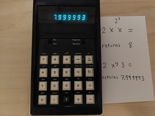
2^3 = 8.

2 [ × ] [ × ] [ = ]  returns 8.   The exact answer.

2 [ f ] [ 6 ] (x^y) 3 [ = ] returns 7.999993

Floating Point Rounding Errors

One drawback of the Electronic Slide rule is the rounding floating point errors.  

70 [ f ] [ ÷ ] (1/x)  returns 0.0142857

Press [ f ] [ ÷ ] (1/x) again returns 70.00007

0.5 [ f ] [ 0 ] (arc) [ 2 ] (cos) returns 59.99999 degrees (it should be 60 degrees)

The forensic test returns 10.4382 (9 sin cos tan arctan arccos arcsin).  

I think the calculator can handle numbers to what the display capacity allows.  There is no internal guard digits to help with accuracy.    

Final Thoughts

I like the feel of the calculator.   The screen has large green numbers which makes the display easy to read.   The keys are are pretty responsive, especially back in the day when it comes to lower-cost calculators in the 1970s (around $100).  

I am not the biggest fan of the negative number indicator, the Rockwell 61R has a negative sign.  Not a deal breaker, though.  The good thing is that red indicator light is bright.  

The Slide Rule is great for fans of Chain Mode (non-algebraic mode).   

If you buy one be sure that:  the charging cord and rechargeable batteries are included and in good working order or the calculator is modified to work on regular AA batteries.

I like how the manual goes in depth with the operations and its library of applications.  

Sources:

Download the manual from Katie Wasserman's Page:  

Sears Electronic Slide Rule:  

https://www.wass.net/manuals/Sears%20Slide%20Rule.pdf

Rockwell 61R:

https://www.wass.net/manuals/Rockwell%2061R.pdf

calculator.org's page on the  Sears Electronic Slide Rule (retrieved July 2, 2023):

https://www.calculator.org/calculators/Sears_Electronic_Slide_Rule.html

Eddie

All original content copyright, © 2011-2023.  Edward Shore.   Unauthorized use and/or unauthorized distribution for commercial purposes without express and written permission from the author is strictly prohibited.  This blog entry may be distributed for noncommercial purposes, provided that full credit is given to the author.