AOS Calculators: Duplicating a Value Without Retyping It

AOS Calculators: Duplicating a Value Without Retyping It

Note: The following applies to scientific classic calculators who operate under the algebraic operating system (AOS) (that is what Texas Instrument’s calls it). I tested this procedure with the following calculators: TI-30X ECO, HP 10bII+ (Algebraic mode), and Casio fx-260 Solar.

Introduction: Going Back to 1976

Imagine it is 1976 and you have have an SR-56 from Texas Instruments. Here is what an SR-56 looks like: http://www.datamath.org/Sci/WEDGE/ZOOM_SR-56.htm

You are tasked to calculate 1.401103287^1.401103287 and do not want to write the number twice. According to page 53 of the SR-56 manual, one approach is to key in:

1.401103287 [ y^x ] [ CE ] [ = ]

Result: 1.604057054

For that particular calculator, SR-56, pressing [ CE ] once stores the number in the display as the second operand allowing the value to duplicated without having to retype the number.

If we tried that on a modern TI-30Xa/TI-30 ECO RS, the display would clear to zero instead of showed the previous number.

However, there are a few tricks we can employ to achieve the similar result.

Trick 1: Pressing the Reciprocal Key Twice

As long as the number in the display is nonzero, pressing [ 1/x ] [ 1/x ] registers the number in the display for as a second operand. In calculators operating in AOS, executing one-argument functions only operate and effect the number in the display only.

Pressing [ 1/x ] takes the reciprocal of the number and registers the number in the display. Pressing [ 1/x ] again returns the number.

**The keystrokes omits any [ 2^nd ] or [ SHIFT ] keys.

Example 1:

Expression: x * log x

Keystrokes: x [ × ] [ 1/x ] [ 1/x ] [ LOG ] [ = ]

5.8 * log 5.8

Keystrokes: 5.8 [ × ] [ 1/x ] [ 1/x ] [ LOG ] [ = ]

Result: 4.427882363

Example 2:

Expression: x^x

Keystrokes: x [ y^x ] [ 1/x ] [ 1/x ] [ = ]

3.088 ^ 3.088

Keystrokes: 3.088 [ y^x ] [ 1/x ] [ 1/x ] [ = ]

Result: 32.51797379

Example 3:

Expression: x * sin x

Keystrokes: x [ × ] [ 1/x ] [ 1/x ] [ SIN ] [ = ]

50° * sin 50°

Keystrokes: ([DRG] to DEG/[ MODE ] (DEG))

50 [ × ] [ 1/x ] [ 1/x ] [ SIN ] [ = ]

Result: 38.30222216

4^4 + 1 / (3^3)

Keystrokes:

4 [ y^x ] [ 1/x ] [ 1/x ] [ + ]

[ ( ] 3 [ y^x ] [ 1/x ] [ 1/x ] [ ) ] [ 1/x ] [ = ]

Result: 256.037037

If the calculator has a cube function (x^3), we can execute this keystroke:

4 [ y^x ] [ 1/x ] [ 1/x ] [ + ]

[ ( ] 3 [ x^3 ] [ ) ] [ 1/x ] [ = ]

Trick 2: Inverse Function Trick

This trick extends the reciprocal trick to include a function that acts on two (and theoretically more) “reversible” functions. This trick applies to the expressions with the following format:

f(x) OP g(x)

f(x)	f^-1(x)	f(x)	f^-1(x)	f(x)	f^-1(x)
SIN	SIN^-1	e^x	LN	X^3	∛
COS	COS^-1	LN	e^x	∛	X^3
TAN	TAN^-1	10^x	LOG	Hyperbolic	Inverse Hyperbolic
SIN^-1	SIN	LOG	10^x	Inverse Hyperbolic	Hyperbolic
COS^-1	COS	X^2	√
TAN^-1	TAN	√	X^2

OP covers the arithmetic operations: [ + ], [ - ], [ × ], [ ÷ ], [ y^x ], and [ y^(1/x) ]

The general keystroke sequence is: x [ f(x) ] [ OP ] [ f^-1(x) ] [ g(x) ] [ = ]

Let’s illustrate this with a few examples. Assume the calculator is in degrees mode.

Example 1:

sin 40° * cos 40°

f(x) = sin x, f^-1(x) = sin^-1 x, g(x) = cos x

Keystrokes: 40 [ SIN ] [ × ] [ SIN^-1 ] [ COS ] [ = ]

Result: 0.492403877

Example 2:

tan 32° * sin 32°

f(x) = tan x, f^-1(x) = tan^-1 x, g(x) = sin x

Keystrokes: 32 [ TAN ] [ × ] [ TAN^-1 ] [ SIN ] [ = ]

Result: 0.331130307

Example 3:

log 881 * ln 881

f(x) = log x, f^-1(x) = 10^x, g(x) = ln x

Keystrokes: 881 [ LOG ] [ × ] [ 10^x ] [ LN ] [ = ]

Result: 19.97005314

Example 4:

e^3.5 / √3.5

f(x) = e^x, f^-1(x) = ln x, g(x) = √x

Keystrokes: 3.5 [ e^x ] [ ÷ ] [ LN ] [ √ ] [ = ]

Result: 17.70095363

Example 5:

√4.555 + e^4.555

f(x) = √x, f^-1(x) = x^2, g(x) = e^x

Keystrokes: 4.555 [ √ ] [ + ] [ x^2 ] [ e^x ] [ = ]

Result: 97.24099983

The inverse function “recovers and registers” the original x. It’s kind of simulating the LAST x feature on RPN calculators.

Sources

Datamath. “Texas Instruments SR-56“ December 5, 2001. http://www.datamath.org/Sci/WEDGE/SR-56.htm

Texas Instruments. Programmable Slid-Rule Calculator SR-56: Owner’s Manual. Dallas, TX. 1976

Eddie

All original content copyright, © 2011-2025. Edward Shore. Unauthorized use and/or unauthorized distribution for commercial purposes without express and written permission from the author is strictly prohibited. This blog entry may be distributed for noncommercial purposes, provided that full credit is given to the author.

All posts are 100% generated by human effort.  The author does not use AI engines and never will.

TI-30Xa Algorithms: RLC Series Circuit

TI-30Xa Algorithms: RLC Series Circuit

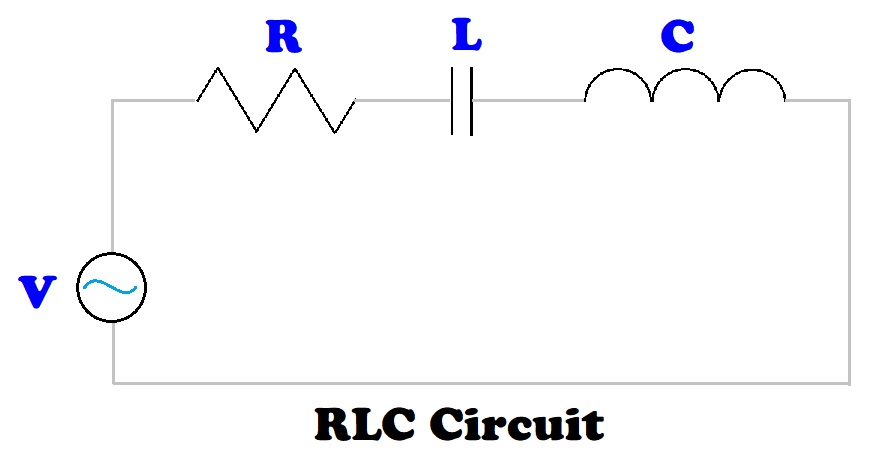
The task is to calculate the total impedance and phase angle for an RLC circuit in a series. An RLC circuit contains a resistor ( R ), an inductor ( L ), and a capacitor ( C ) , all powered by a voltage supply. The resistor, inductor, and capacitor are all in a single path.

The three elements are measured in the following units:

Resistor ( R ): Ohms ( Ω )

Inductor ( L ): Henry ( H )

Capacitor ( C ): Farads ( F )

The impedance for the RLC circuit is calculated by:

Z = √( R^2 + ( (2 * π * f * L) - 1 / (2 * π * f * C) )^2 )

The phase angle is calculated by:

θ = arctan( ( (2 * π * f * L) - 1 / (2 * π * f * C) ) / R )

where: f = frequency in Hertz (Hz)

We can use the rectangular to polar conversion function (R>P) to calculate both the impedance and phase angle.

x = R

y = (2 * π * f * L) - 1 / (2 * π * f * C)

If we have an RL circuit, with no capacitor, then C = 0.

If we have an RC circuit, with no inductor, then L = 0.

If we have an LC circuit, with no resistor, then R = 0.

TI-30Xa Algorithm – RLC Circuit

Step 1: Store resistance in Memory 1.

R [ STO ] 1

Step 2: Calculate angular frequency, ω = 2 * π * f, store in memory 3.

2 [ × ] [ π ] [ × ] f [ = ] [ STO ] 3

Step 3: Calculate (2 * π * f * L) - 1 / (2 * π * f * C)

[ RCL ] 3 [ × ] L [ - ] [ ( ] [ RCL ] 3 [ × ] C [ ) ] [ 1/x ] [ = ] [ STO ] 2

If we have an RL circuit, Steps 2 and 3 can be shortened to:

2 [ × ] [ π ] [ × ] f [ × ] L [ = ] [ STO ] 2

If we have an RC circuit, Steps 2 and 3 can be shortened to:

[ ( ] 2 [ × ] [ π ] [ × ] f [ × ] C [ ) ] [ 1/x ] [ +/- ] [ = ] [ STO ] 2

Step 4: Calculate Impedance and Phase Angle:

[ RCL ] 1 [ 2^nd ] [ π ] (x<>y) [ RCL ] 2 [ 2^nd ] [ - ] (R>P)

What is shown: (r) Impedance

Press [ 2^nd ] [ π ] (x<>y) for phase angle (θ)

Examples

Example 1: RLC Series Circuit

R = 50 Ω

L = 3.8 H

C = 0.7 F

f = 40 Hz

Step 1: Store resistance in Memory 1.

50 [ STO ] 1

Step 2: Calculate angular frequency, ω = 2 * π * f, store in memory 3.

2 [ × ] [ π ] [ × ] 40 [ = ] [ STO ] 3 (251.3274123)

Step 3: Calculate (2 * π * f * L) - 1 / (2 * π * f * C)

[ RCL ] 3 [ × ] 3.8 [ - ] [ ( ] [ RCL ] 3 [ × ] 0.0007 [ ) ] [ 1/x ] [ = ] [ STO ] 2

(949.36000616)

Step 4: Calculate Impedance and Phase Angle:

[ RCL ] 1 [ 2^nd ] [ π ] (x<>y) [ RCL ] 2 [ 2^nd ] [ - ] (R>P)

Impedance: 950.6758262

Phase Angle: 86.9851854°

Example 2: RLC Series Circuit

R = 450 Ω

L = 1.15 H

C = 3.5 μF = 3.5 * 10^-6 F

f = 60 Hz

Step 1: Store resistance in Memory 1.

450 [ STO ] 1

Step 2: Calculate angular frequency, ω = 2 * π * f, store in memory 3.

2 [ × ] [ π ] [ × ] 60 [ = ] [ STO ] 3 (376.9911184)

Step 3: Calculate (2 * π * f * L) - 1 / (2 * π * f * C)

[ RCL ] 3 [ × ] 1.15 [ - ] [ ( ] [ RCL ] 3 [ × ] 3.5 [ EE ] 6 [ +/- ] [ ) ] [ 1/x ] [ = ] [ STO ] 2

(-324.3408952)

Step 4: Calculate Impedance and Phase Angle:

[ RCL ] 1 [ 2^nd ] [ π ] (x<>y) [ RCL ] 2 [ 2^nd ] [ - ] (R>P)

Impedance: 554.7044405

Phase Angle: -35.78246242°

Source

“Impedance and Complex Impedance” Electronics Tutorials. AspenCore, Inc. 2024. Retrieved October 7, 2024. https://www.electronics-tutorials.ws/accircuits/impedance.html

This wraps up the TI-30Xa Algorithm Series. Next up will be a series on the Casio fx-991CW.

I want to wish you all a Happy New Year and a prosperous, sane, and happy 2025! Be safe, everyone, it’s a very crazy world we live in.

Eddie

All original content copyright, © 2011-2024. Edward Shore. Unauthorized use and/or unauthorized distribution for commercial purposes without express and written permission from the author is strictly prohibited. This blog entry may be distributed for noncommercial purposes, provided that full credit is given to the author.

TI-30Xa and HP 12C: Linear Interpolation

TI-30Xa and HP 12C: Linear Interpolation

Introduction

Given two points (x0, y0) and (x1, y1), and a point, x, we can easily estimate the y coordinate:

y = y0 + (x – x0) * (y1 – y0) / (x1 – x0)

Note that the slope of the line is:

m = (y1 – y0) / (x1 – x0)

This works the best when x is relatively real close to x0 and x1.

Fun fact, the y-intercept, where x = 0 can be calculated as:

b = y0 – x0 * m

TI-30Xa Algorithm: Linear Interpolation

This algorithm will require to enter information only once.

Store the following points:

x0 [ STO ] 1

y0 [ STO ] 2

Predict y:

[ ( ] x [ - ] [ RCL ] 1 [ ) ] [ × ] [ ( ] y1 [ - ] [ RCL ] 2 [ ) ] [ ÷ ] [ ( ] x1 [ - ] [ RCL ] 1 [ ) ] [ + ] y0 [ = ]

HP 12C Algorithm: Linear Interpolation

It turns out that we can use the linear regression functions for linear interpolation. Entering two points for linear regression will create a perfect line (with the correlation of 1 or -1). The algorithm presented is for the HP 12C, and a algorithm for other calculators can easily be made.

Keystrokes:

Enter (x0, y0) and (x1, y1):

[ f ] [ Clx ] (CLEAR FIN)

y0 [ ENTER ] x0 [ Σ+ ]

y1 [ ENTER ] x1 [ Σ+ ]

To calculate y:

x [ g ] [ 2 ] (y-hat, r)

Examples

Examples	X0	Y0	X1	Y1	X (Input)	Y (Output)
1	10	4.95	12	5.06	11	5.0050
2	21	48,057	23	52,165	22	50,111
3	1000	97.7	2000	94.2	1500	95.95

Source

“Linear interpolation” Wikipedia. Was Edited August 27, 2024. Retrieved September 4, 2024. https://en.wikipedia.org/wiki/Linear_interpolation

Until next time, as we head into the final month of 2024,

Eddie

All original content copyright, © 2011-2024. Edward Shore. Unauthorized use and/or unauthorized distribution for commercial purposes without express and written permission from the author is strictly prohibited. This blog entry may be distributed for noncommercial purposes, provided that full credit is given to the author.

TI 30Xa Algorithm: Acceleration, Velocity, Speed

TI 30Xa Algorithm: Acceleration, Velocity, Speed

Introduction and Algorithm

Given the acceleration (α), initial velocity (v0), and initial position (p0) of an object on a 2D plane, calculate velocity and position at time T.

Assuming that acceleration is constant, the equations are:

Acceleration: A = α

Velocity: V = α * t + v0

Position: P = α / 2 * t^2 + v0 * t + p0

With some simplification, we can simplify the work flow:

( I )

A = α

( II )

V = α * t + v0

V = A * t + v0 (II)

( III )

P = α / 2 * t^2 + v0 * t + p0

P = t * ( α / 2 * t + v0 ) + p0

P = t * ( α / 2 * t + 2 * v0 / 2 ) + p0

P = t * ( (α * t + 2 * v0) / 2 ) + p0

P = t / 2 * ( α * t + 2 * v0 ) + p0

P = t / 2 * ( α * t + v0 + v0 ) + p0

P = t * (V + v0) / 2 + p0

( I ): A = α

( II ): V = A * t + v0

( III ): P = t * (V + v0) / 2 + p0

Key Strokes:

1. Store the time T in Memory 1 ( T [ STO ] 1 )

2. Store the initial velocity in Memory 2 ( v0 [ STO ] 2 )

3. Enter the acceleration constant, α, press [ = ]

4. Calculate the velocity at time T: [ × ] [ RCL ] 1 [ + ] [ RCL ] 2 [ = ]

5. Calculate the position at time T: [ + ] [ RCL ] 2 [ = ] [ × ] [ RCL ] 1 [ ÷ ] 2 [ + ] p0 [ = ]

Examples

Example 1:

α = 1.3

v0 = 0

p0 = 0

T = 10

1. 10 [ STO ] 1

2. 0 [ STO ] 2

3. Acceleration: 1.3 [ = ]

4. Velocity: [ × ] [ RCL ] 1 [ + ] [ RCL ] 2 [ = ] (Result: 13)

5. Position: [ + ] [ RCL ] 2 [ = ] [ × ] [ RCL ] 1 [ ÷ ] 2 [ + ] 0 [ = ] (Result: 65)

Example 2:

α = -9.80665

v0 = 0

p0 = 10000

T = 30

1. 30 [ STO ] 1

2. 0 [ STO ] 2

3. Acceleration: 9.80665 [ +/- ] [ = ]

4. Velocity: [ × ] [ RCL ] 1 [ + ] [ RCL ] 2 [ = ] (Result: -294.1995)

5. Position: [ + ] [ RCL ] 2 [ = ] [ × ] [ RCL ] 1 [ ÷ ] 2 [ + ] 10000 [ = ] (Result: 5587.0075)

Example 3:

α = -0.05

v0 = 10

p0 = 20

T = 15

1. 15 [ STO ] 1

2. 10 [ STO ] 2

3. Acceleration: 0.05 [ +/- ] [ = ]

4. Velocity: [ × ] [ RCL ] 1 [ + ] [ RCL ] 2 [ = ] (Result: 9.25)

5. Position: [ + ] [ RCL ] 2 [ = ] [ × ] [ RCL ] 1 [ ÷ ] 2 [ + ] 20 [ = ] (Result: 164.375)

Example 4:

α = 4.26

v0 = 1.8

p0 = 0

T = 5

1. 5 [ STO ] 1

2. 1.8 [ STO ] 2

3. Acceleration: 4.26 [ = ]

4. Velocity: [ × ] [ RCL ] 1 [ + ] [ RCL ] 2 [ = ] (Result: 23.1)

5. Position: [ + ] [ RCL ] 2 [ = ] [ × ] [ RCL ] 1 [ ÷ ] 2 [ + ] 0 [ = ] (Result: 62.25)

Hope you find this useful.

Happy Halloween, Everyone!

Eddie

All original content copyright, © 2011-2024. Edward Shore. Unauthorized use and/or unauthorized distribution for commercial purposes without express and written permission from the author is strictly prohibited. This blog entry may be distributed for noncommercial purposes, provided that full credit is given to the author.