TI-Nspire: Templates to Plot Functions, Parametric Equations, and Sequences

 TI-Nspire:  Templates to Plot Functions, Parametric Equations, and Sequences

Introduction

The following are sample templates to plot functions in the form of y=f(x), parametric equations (x(t), y(t)), and one-level deep recurrence relations.

I used a while loop instead of a for loop because I tend to always use for loops, and working with integer objects can be quite difficult for non-Python experts like me.  

The equations will be defined inside the script instead of having the user enter the script.  .   I am using the TI-NSpire CX II software 5.2.0771.  I have programmed this with the TI-Nspire CX CAS software, but it should work on the non-CAS version.  

As far as entering numbers at the input prompt, I have to enter approximations for π (which is approximately 3.1415926535).  

The list.append(value) or list.append(list) adds the elements to the end of the list and the list is automatically saved.  

The graphic commands uses a TI-specific module ti_plotlib.  I have a lot of pleasure working with this module, with commands for clearing the graphic screen, automatically sizing the window, plotting the axes, with or without the numeric numeric endpoints, and set a color with RGB codes (any color you want).  

You can download the file here:  https://drive.google.com/file/d/1k_3lTVK5KK1ACXrVxemSWz_g-l8Nn62A/view?usp=sharing

The text of the scripts are presented below.

Plotting Functions -   TI-Nspire CX II (CAS) Script:  plotfxnspire.py

from math import *

import ti_plotlib as plt

# EWS 2020-12-28

# define function here

def f(x):

  y=1/(x**2+1)

  return y

# main routine

xa=float(input('start? '))

xb=float(input('stop? '))

n=float(input('n? '))

xc=(xb-xa)/n

# build

xp=xa

yp=f(xp)

xlist=[xp]

ylist=[yp]

while xp<xb:

  xp=xp+xc

  yp=f(xp)

  xlist.append(xp)

  ylist.append(yp)

# plot routine

# clear the screen

plt.cls()

# automatically fits the screen to fit the data

plt.auto_window(xlist,ylist)

# display the axes

# "on" plots axes and endpoints

# "axes" just plots the axes

plt.axes("on")

# select color - use RGB style

# denim blue

plt.color(21,96,189)

# plot the graph

plt.plot(xlist,ylist,".")

plt.show_plot()

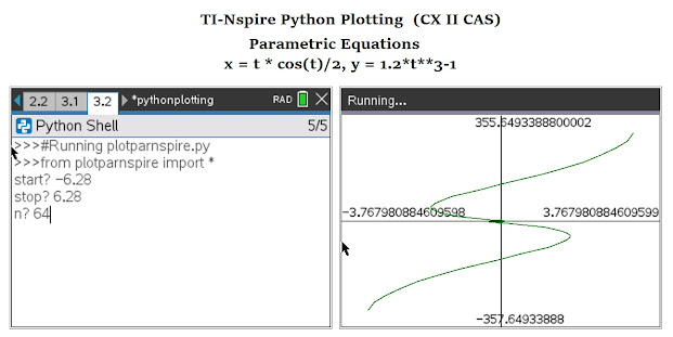
Plotting Parametric Equations -   TI-Nspire CX II (CAS) Script:  plotparnspire.py

from math import *

import ti_plotlib as plt

# EWS 2020-12-28

# define parametric here

def x(t):

  x=t*cos(t)/2

  return x

def y(t):

  y=1.2*t**3-1

  return y

# main routine

ta=float(input('start? '))

tb=float(input('stop? '))

n=float(input('n? '))

tc=(tb-ta)/n

# build

tp=ta

xp=x(tp)

yp=y(tp)

xlist=[xp]

ylist=[yp]

while tp<tb:

  tp=tp+tc

  xp=x(tp)

  yp=y(tp)

  xlist.append(xp)

  ylist.append(yp)

# plot routine

# clear the screen

plt.cls()

# automatically fits the screen to fit the data

plt.auto_window(xlist,ylist)

# display the axes

# "on" plots axes and endpoints

# "axes" just plots the axes

plt.axes("on")

# select color - use RGB style

# mid green

plt.color(0,128,0)

# plot the graph

plt.plot(xlist,ylist,".")

plt.show_plot()

Plotting a Recurrence Relation-   TI-Nspire CX II (CAS) Script:  plotseqnspire.py

Use u for u_n-1.  You should also be able to include n without problems.  

from math import *

import ti_plotlib as plt

# EWS 2020-12-28

# define sequence here, u for u(n-1)

def w(u):

  w=cos(u)+1

  return w

# main routine

ui=float(input('initial? '))

n=float(input('n? '))

# build

xlist=[0]

ylist=[ui]

k=0

while k<n:

  k=k+1

  f=w(k)

  xp=k

  yp=f

  xlist.append(xp)

  ylist.append(yp)

# plot routine

# clear the screen

plt.cls()

# automatically fits the screen to fit the data

plt.auto_window(xlist,ylist)

# display the axes

# "on" plots axes and endpoints

# "axes" just plots the axes

plt.axes("on")

# select color - use RGB style

# orange

plt.color(255,127,39)

# plot the graph

plt.plot(xlist,ylist,".")

plt.show_plot()

Eddie

All original content copyright, © 2011-2021.  Edward Shore.   Unauthorized use and/or unauthorized distribution for commercial purposes without express and written permission from the author is strictly prohibited.  This blog entry may be distributed for noncommercial purposes, provided that full credit is given to the author. 

Numworks: Templates to Plot Functions, Parametric Equations, and Sequences

 Numworks:  Templates to Plot Functions, Parametric Equations, and Sequences

Introduction

The following are sample templates to plot functions in the form of y=f(x), parametric equations (x(t), y(t)), and one-level deep recurrence relations.

I used a while loop instead of a for loop because I tend to always use for loops, and working with integer objects can be quite difficult for non-Python experts like me.  

The equations will be defined inside the script instead of having the user enter the script.  If anyone knows how to use input to enter functions, please let me know.   I am using Numworks software version 14.4.  

As far as entering numbers at the input prompt, I have to enter approximations for π (which is approximately 3.1415926535).  The plot screen is made to fit the y-minimum and y-maximum values within the window.

The list.append(value) or list.append(list) adds the elements to the end of the list and the list is automatically saved.  

The named colors, which is required in matplolib.pyplot, available are:  'black', 'blue', 'brown', 'green', 'grey', 'orange', 'pink', 'purple', 'red', 'white', and 'yellow'.

Plotting Functions -   Numworks Script:  plotfunction.py

from math import *

from matplotlib.pyplot import *

# EWS 2020-12-26

# define function here

def f(x):

  y=1/(x**2+1)

  return y

# main routine

xa=float(input('start? '))

xb=float(input('stop? '))

n=float(input('n? '))

xc=(xb-xa)/n

# build

xp=xa

yp=f(xp)

xlist=[xp]

ylist=[yp]

while xp<xb:

  xp=xp+xc

  yp=f(xp)

  xlist.append(xp)

  ylist.append(yp)

  

# plot routine

# set axes

ya=min(ylist)

yb=max(ylist)

axis((xa,xb,ya,yb))

axis(True)

grid(True)

# select color, type color

ch="blue"

# plot points

plot(xlist,ylist,color=ch)

show()

Plotting Parametric Equations -   Numworks Script:  plotparametric.py

from math import *

from matplotlib.pyplot import *

# EWS 2020-12-26

# define parametric here

def x(t):

  x=t**2-3*t+1

  return x

def y(t):

  y=abs(2*sin(t))

  return y

# main routine

ta=float(input('start? '))

tb=float(input('stop? '))

n=float(input('n? '))

tc=(tb-ta)/n

# build

tp=ta

xp=x(tp)

yp=y(tp)

xlist=[xp]

ylist=[yp]

while tp<tb:

  tp=tp+tc

  xp=x(tp)

  yp=y(tp)

  xlist.append(xp)

  ylist.append(yp)

  

# plot routine

# set axes

xa=min(xlist)

xb=max(xlist)

ya=min(ylist)

yb=max(ylist)

axis((xa,xb,ya,yb))

axis(True)

# select color, type color

ch="red"

# plot points

plot(xlist,ylist,color=ch)

show()

Plotting a Recurrence Relation-   Numworks Script:  plotsequence.py

Use u for u_n-1.  You should also be able to include n without problems.  

from math import *

from matplotlib.pyplot import *

# EWS 2020-12-26

# define parametric here

# u: u(n-1)

def w(u):

  f=sqrt(3*u+1)

  return f

# main routine

ui=float(input('initial? '))

n=float(input('n? '))

# build

xlist=[0]

ylist=[ui]

k=0

while k<n:

  k=k+1

  f=w(k)

  xp=k

  yp=f

  xlist.append(xp)

  ylist.append(yp)

  

# plot routine

# set axes

ya=min(ylist)

yb=max(ylist)

axis((0,n,ya,yb))

axis(True)

# select color, type color

ch="green"

# plot points

plot(xlist,ylist,color=ch)

show()

On tomorrow's blog, January 17, 2021, I am going to present these scripts for the TI-Nspire CX II.   I used the CX CAS software, but this should work on the CX (non-CAS) calculator and software as well.  

Eddie

All original content copyright, © 2011-2021.  Edward Shore.   Unauthorized use and/or unauthorized distribution for commercial purposes without express and written permission from the author is strictly prohibited.  This blog entry may be distributed for noncommercial purposes, provided that full credit is given to the author. 

TI-84 Plus CE: Time Plot of Two Parametric Equations

TI-84 Plus CE:  Time Plot of Two Parametric Equations

Introduction 

The program TIMEPLOT animates two parametric plots. 

TI-84 Plus Program TIMEPLOT
(237 bytes)

"EWS 2019-04-22"
Param
PlotsOff
FnOff
Input "T START:",A
Input "T STOP:", B
Input "T STEP:", S
int((B-A)/S) → N
A → T: {X1T} → L1 : {Y1T} → L2
{X2T} → L3: {Y2T} → L4
For(I,2,N)
A + S*(I-1) → T
augment(L1, {X1T}) → L1
augment(L2, {Y1T}) → L2
augment(L3, {X2T}) → L3
augment(L4, {Y2T}) → L4
Plot1(Scatter, L1, L2, □, BLUE)
Plot2(Scatter, L3, L4, □, GREEN)
DispGraph 
Wait 1
End

Example

X1T = 2 SIN T
Y1T = 3 SIN T

X2T = SIN (T^2/4)
Y2T = 1/2 * COS(T^2/8)

T START: 0
T STOP: 4 * π
T STEP: π / 24

Eddie

All original content copyright, © 2011-2019.  Edward Shore.   Unauthorized use and/or unauthorized distribution for commercial purposes without express and written permission from the author is strictly prohibited.  This blog entry may be distributed for noncommercial purposes, provided that full credit is given to the author.

How to Rotate Graphs

How to Rotate Graphs

Introduction

The key is to use parametric equations in our rotation.  Using the rotation angle θ, the rotation matrix is:

R = [ [ cos θ, -sin θ ] [ sin θ, cos θ ] ]

With the equations x(t), y(t) set as the matrix:

M = [ [ x(t) ] [ y(t) ] ]

The rotated graph is:

[ [ x’(t) ] [ y’(t) ] ] = R * M

Where:

x’(t) = x(t) * cos θ – y(t) * sin θ

y’(t) = x(t) * sin θ + y(t) * cos θ

Rotation the Function y = f(x)

Let x = t and set the parametric functions:

x(t) = t

y(t) = f(t)

Rotating the Polar Equation r = f(t)  (where t = θ)

1.  Solve for t.

2.  Substitute r and t in the following equations:

  x(t) = r * cos t

  y(t) = r * sin t

3.  Simplify as needed.

Some trigonometric properties:

sin^2 ϕ + cos^2 ϕ = 1

sin(2*ϕ) = 2 * cos ϕ * sin ϕ

cos(2*ϕ) = 2 * cos^2 ϕ – 1

sin(acos ϕ) = cos(asin ϕ) = √(1 – ϕ^2)

Please refer to this link for additional details:  http://edspi31415.blogspot.com/2013/01/converting-polar-equations-to.html

   

Rotation Matrices for Certain Angles

Angle 30°, π/6:  R = [ [ √3/2, -1/2 ] [ 1/2, √3/2 ] ]

Angle 45°, π/4:  R = [ [ √2/2, -√2/2 ] [ √2/2, √2/2 ] ]

Angle 60°, π/3:  R = [ [ 1/2, -√3/2 ] [ √3/2, 1/2 ] ]

Angle 90°, π/2:  R = [ [ 0, -1 ] [ 1, 0 ] ]

Angle 120°, 2π/3:  R = [ [ -1/2, -√3/2 ] [ √3/2, -1/2 ] ]

Angle 135°, 3π/4:  R = [ [ -√2/2, -√2/2 ] [ √2/2, -√2/2 ] ]

Angle 150°, 5π/6:  R = [ [ -√3/2, -1/2 ] [ 1/2, -√3/2 ] ]

Angle 180°, π:  R = [ [ -1, 0 ] [ 0, -1 ] ]

Angle 210°, 7π/6:  R = [ [ -√3/2, 1/2 ] [ -1/2, -√3/2 ] ]

Angle 225°, 5π/4:  R = [ [ -√2/2, √2/2 ] [ -√2/2, -√2/2 ] ]

Angle 240°, 4π/3:  R = [ [ -1/2, √3/2 ] [ -√3/2, -1/2 ] ]

Angle 270°, 3π/2:  R = [  [ 0, 1 ] [ -1, 0 ] ]

Angle 300°, 5π/3:  R = [ [ 1/2, √3/2 ] [ -√3/2, 1/2 ] ]

Angle 315°, 7π/4:  R = [ [ √2/2, √2/2 ] [ -√2/2, √2/2  ] ]

Angle 330°, 11π/6:  R = [ [ √3/2, 1/2 ] [ -1/2, √3/2  ] ]

Examples

Each example is followed by a graph of the original equation (blue) and the rotated equations (red).  I used a Casio fx-CG 50 for the screen shots.

Example 1:  y = 3*x^2, rotate 90°

We have a function in the form of y = f(x).  Let’s transfer the function to parametric form, first by assigning x = t and y = 3*t^2.  Angle mode is in radians.

With 90°, the rotation matrix is:  R = [ [ 0, -1 ] [ 1, 0 ] ]

The transformed equations are:

[ [ 0, -1 ] [ 1, 0 ] ] * [ [ t ] [ 3*t^2 ] ] = [ [ -3*t^2 ] [ t ] ]

Rotated Equations:  x’(t) = -3*t^2, y’(t) = t

Example 2:  x = t^3, y = 2*t – 1, rotate 270°

We have the equations in parametric form.  We’ll need the rotation matrix, where:

R = [  [ 0, 1 ] [ -1, 0 ] ]

[  [ 0, 1 ] [ -1, 0 ] ] * [ [ t^3 ] [ 2*t – 1 ] ] = [ [ 2*t – 1 ] [ -t^3 ] ]

Rotated Equations:  x’(t) = 2*t – 1, y’(t) = -t^3

Example 3:  x = sin t, y = e^t, rotate 135°

The rotation matrix is R = [ [ -√2/2, -√2/2 ] [ √2/2, -√2/2 ] ]

Rotated Equations:  x’(t) = -√2/2 * (sin t + e^t), y’(t) = √2/2 * (sin t – e^t)

Example 4:  r = 2 θ, rotate 60°

The parametric form is x(t) = 2 * t * cos t, y(t) = 2 * t * sin t

The rotation matrix is R = [ [ 1/2, -√3/2 ] [ √3/2, 1/2 ] ]

Rotated Equations: x’(t) = t * cos t - √3 * t * sin t, y’(t) = t * sin t + √3 * t * cos t

Eddie

This blog is property of Edward Shore, 2017

HP Prime Geometry App Tutorial Part 5: Plotting Functions and Differential Equations

HP Prime Geometry App Tutorial Part 5:  Plotting Functions and Differential Equations

The Geometry App can plot functions, parametric functions, polar functions, sequences, implicit statements, slope-field and ordinary differential equations, lists, and designate sliders.   

In this lesson, we will demonstrate three types of plots.   For the purpose of the tutorial, clear the Plot screen before each example.

Plotting Functions ( y = f(x))

Plot y = e^x + 1.

1.  Press (Cmds), 6 for Plot, 1 for Function. 

2.  Type e^(x) + 1.  Press (OK).

Use the lowercase x.  The format is plotfunc( y(x) ).

Plot an Ordinary Differential Equation  (y’ = dy/dx = f(x,y))

Plot y’ = y*e^x +1 with the initial condition (1,1).

1.  Press (Cmds), 6 for Plot, 7 for ODE.

2.  Type y*e^(x)+1.   Note that x and y are in lowercase.

3.  Press [ , ] and type [x,y].   Here you designate which variable is independent and which is dependent.

4.  Press [ , ] and type  [1,1].  This is your initial conditions.  Press (OK), 

The entire format is plotode( f(x,y),  [x, y], [x0, y0])

Plot a Parametric Equation  ( x(t) + i*y(t) where i = √-1)

Plot x = 3t + 1, y = 2t – 1.   The format to be used is (3t + 1) + i*(2t -1).

‘1. Press (Cmds), 6 for Plot, 2 for Parametric.

‘2. Type (3t + 1) + i*(2t -1) and press ( OK ).

The entire format is plotparam( x(t) + i*y(t), var = tbeg..tend, tstep=step).  The t is in lowercase and the last two arguments, interval and step, are optional.

In Part 6 we’ll be plotting and working with polygons.   Thanks and take care,

Eddie

This blog is property of Edward Shore.  2015. 

Converting Polar Equations to Parametric Equations

Good Sunday!

This blog will show how to transform polar equations, in the form of r(θ) to a pair of parametric equations, x(t) and y(t).

---

Tools We Need

x = r * cos θ
y = r * sin θ

Let θ = t.

---

For each example, we will change each polar equation and display a graph for each form. The polar form, colored blue, is on top; the parametric form, in red, is on the bottom. (A TI nSpire-CX is used for the pictures)

Example (I):

r = 2*θ

Then θ = r/2 and let θ = t.

x = r * cos t
x = 2 * t * cos(r/2)
x = 2 * t * cos((2*t)/2)
x = 2 * t * cos t

Similarly,

y = r * sin t
y = 2 * t * sin(r/2)
y = 2 * t * sin t

To summarize:
r = 2*θ

is equivalent to

x = 2 * t * cos t
y = 2 * t * sin t

Example (II):

r = e^(2 * θ)

Then θ = 1/2 * ln r and let θ = t.

And...

x = r * cos t
x = e^(2*t) * cos(1/2 * ln r)
x = e^(2*t) * cos(1/2 * ln(e^(2*t)))
x = e^(2*t) * cos(1/2 * 2 * t)
x = e^(2*t) * cos t

y = r * sin t
y = e^(2*t) * sin(1/2 * ln r)
y = e^(2*t) * sin(1/2 * ln(e^(2*t)))
y = e^(2*t) * sin t



To summarize:
r = e^(2*θ)

is equivalent to:

x = e^(2*t) * cos t
y = e^(2*t) * sin t

Example (III):

r = 2 cos θ

Then:

θ = arccos(r/2) = cos⁻¹(r/2)

Then, with θ=t...

x = r * cos t
x = 2 * cos t * cos(cos⁻¹(r/2))
x = 2 * cos t * cos(cos⁻¹(2*cos(t)/2))
x = 2 * cos t * cos t
x = 2 * cos² t

And... (some trigonometric identities are required)

y = r * sin t
y = 2 * cos t * sin(cos⁻¹(r/2))

Note: sin(cos⁻¹ x) = √(1 - x²)

y = 2 * cos t * √((1 - (r/2)²)
y = 2 * cos t * √(1 - r²/4)
y = 2 * cos t * √(1 - (4 cos² t)/4)
y = 2 * cos t * √(1 - cos² t)

Note: sin² x + cos² x = 1

y = 2 * cos t * sin t

Note: sin(2*x) = 2 * cos x * sin x

y = sin (2*t)

To Summarize:
r = 2 cos θ

is equivalent to:

x = 2 * cos² t
y = sin (2*t)

Until next time, take care!

Eddie


This blog is property of Edward Shore. 2013