Simple Generating Functions

 Generating Functions 

Generating a Sequence Via a Function

A generating function, g(x), can be expressed as a power series polynomial.  The coefficients of such polynomials make up the generating sequence.

g(x) = Σ( c_k * x^k, k=0 to ∞) = c_0 + c_1 * x + c_2 * x^2 + c_3 * x^3 + ....

The generated sequence is {c_0, c_1, c_2, c_3, ... }.

A simple approach is find the Maclaurin Series (Taylor Series about the point 0) of g(x).

Example:

g(x) = 2 ÷ (1 - 3*x)

The Maclaurin Series of g(x) is:

2 + 6*x + 18*x^2 + 54*x^3 + 162*x^4 + 486*x^5 + ...

with the sequence of { 2, 6, 18, 54, 162, 486 ... }

Some Simple Generating Functions

1 ÷ (1 - x) = 1 + x + x^2 + x^3 + x^4 + ....

b ÷ (1 - x) = b + b + b^2 + b^3 + b^4 + ....

1 ÷ (1 - a*x) = 1 + a*x + a^2*x^2 + a^3*x^3 + a^4*x^4 + ....

1 ÷ (1 - x)^2 = 1 + 2*x + 3*x^2 + 4*x^3 + 5*x^4 + ....

1 ÷ (1 + x) = 1 - x + x^2 - x^3 + x^4 - x^5 + ....

(as pictures the size of 3" x 5" index cards:  let me know if you want more posts like this - Eddie)

All original content copyright, © 2011-2021.  Edward Shore.   Unauthorized use and/or unauthorized distribution for commercial purposes without express and written permission from the author is strictly prohibited.  This blog entry may be distributed for noncommercial purposes, provided that full credit is given to the author. 

Numworks: Update to Software Version 15.5

Numworks: Update to Software Version 15.5 

On May 10, 2021 updated their software of the Numworks graphing calculator to Version 15.5.0.   

New Features

Some of the new features include:

Calculation Mode: 

*  The Calculation mode gets a new section:  Vectors.  The available functions are dot, cross, and norm.  

*  The ref and rref functions are added to the Matrices section.

*  When the results is a matrix, we can go up into the history, select the three dots next the matrix.  This gives us the additional results:  determinant*, inverse*, row echelon form, reduce row echelon form, and trace* (*for square matrices only)

* Like functions, sequences can be evaluated from outside the respective graphing (Sequence) mode.  

Functions Mode:

*  The graph can be auto-scaled.  

Other:

*  The gcd and lcm commands can accept more than two arguments.  

*  Even though they can't be used in algebraic expressions, the °C and °F units are added to the units menu.  

*  Many imperial (United States) units are added such as ft, acre, lb, and gal.  

You can find all the details here:

https://workshop.numworks.com/firmwares

I have to remember than Numworks does a lot more than Python.  

How to Upgrade Your Numworks Calculator

1.  Go to the Numworks website.  It is recommended that you use Google Chrome.

2.  Plug in your calculator by USB port.   The website should detect your calculator automatically.

3.  Under your name, click on My Devices and click on the (Update my device) button.  The update process takes approximately less than one minute.

4.  Once the update is done, you can unplug your calculator.

Version 15.5.0 (3e071a5)

How to Check Your Numwork's Software Version

There are two ways that I know of:

1.  Plug your calculator by USB and go to the Numworks website.  Under your name, select My Devices.

- or -

2.  On the calculator, press the Home key, scroll down to Settings.  Press [ EXE ].  Scroll down and select About.

That's it!  Enjoy,

Eddie

All original content copyright, © 2011-2021.  Edward Shore.   Unauthorized use and/or unauthorized distribution for commercial purposes without express and written permission from the author is strictly prohibited.  This blog entry may be distributed for noncommercial purposes, provided that full credit is given to the author. 

TI-Nspire: Templates to Plot Functions, Parametric Equations, and Sequences

 TI-Nspire:  Templates to Plot Functions, Parametric Equations, and Sequences

Introduction

The following are sample templates to plot functions in the form of y=f(x), parametric equations (x(t), y(t)), and one-level deep recurrence relations.

I used a while loop instead of a for loop because I tend to always use for loops, and working with integer objects can be quite difficult for non-Python experts like me.  

The equations will be defined inside the script instead of having the user enter the script.  .   I am using the TI-NSpire CX II software 5.2.0771.  I have programmed this with the TI-Nspire CX CAS software, but it should work on the non-CAS version.  

As far as entering numbers at the input prompt, I have to enter approximations for π (which is approximately 3.1415926535).  

The list.append(value) or list.append(list) adds the elements to the end of the list and the list is automatically saved.  

The graphic commands uses a TI-specific module ti_plotlib.  I have a lot of pleasure working with this module, with commands for clearing the graphic screen, automatically sizing the window, plotting the axes, with or without the numeric numeric endpoints, and set a color with RGB codes (any color you want).  

You can download the file here:  https://drive.google.com/file/d/1k_3lTVK5KK1ACXrVxemSWz_g-l8Nn62A/view?usp=sharing

The text of the scripts are presented below.

Plotting Functions -   TI-Nspire CX II (CAS) Script:  plotfxnspire.py

from math import *

import ti_plotlib as plt

# EWS 2020-12-28

# define function here

def f(x):

  y=1/(x**2+1)

  return y

# main routine

xa=float(input('start? '))

xb=float(input('stop? '))

n=float(input('n? '))

xc=(xb-xa)/n

# build

xp=xa

yp=f(xp)

xlist=[xp]

ylist=[yp]

while xp<xb:

  xp=xp+xc

  yp=f(xp)

  xlist.append(xp)

  ylist.append(yp)

# plot routine

# clear the screen

plt.cls()

# automatically fits the screen to fit the data

plt.auto_window(xlist,ylist)

# display the axes

# "on" plots axes and endpoints

# "axes" just plots the axes

plt.axes("on")

# select color - use RGB style

# denim blue

plt.color(21,96,189)

# plot the graph

plt.plot(xlist,ylist,".")

plt.show_plot()

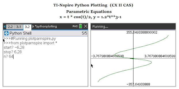
Plotting Parametric Equations -   TI-Nspire CX II (CAS) Script:  plotparnspire.py

from math import *

import ti_plotlib as plt

# EWS 2020-12-28

# define parametric here

def x(t):

  x=t*cos(t)/2

  return x

def y(t):

  y=1.2*t**3-1

  return y

# main routine

ta=float(input('start? '))

tb=float(input('stop? '))

n=float(input('n? '))

tc=(tb-ta)/n

# build

tp=ta

xp=x(tp)

yp=y(tp)

xlist=[xp]

ylist=[yp]

while tp<tb:

  tp=tp+tc

  xp=x(tp)

  yp=y(tp)

  xlist.append(xp)

  ylist.append(yp)

# plot routine

# clear the screen

plt.cls()

# automatically fits the screen to fit the data

plt.auto_window(xlist,ylist)

# display the axes

# "on" plots axes and endpoints

# "axes" just plots the axes

plt.axes("on")

# select color - use RGB style

# mid green

plt.color(0,128,0)

# plot the graph

plt.plot(xlist,ylist,".")

plt.show_plot()

Plotting a Recurrence Relation-   TI-Nspire CX II (CAS) Script:  plotseqnspire.py

Use u for u_n-1.  You should also be able to include n without problems.  

from math import *

import ti_plotlib as plt

# EWS 2020-12-28

# define sequence here, u for u(n-1)

def w(u):

  w=cos(u)+1

  return w

# main routine

ui=float(input('initial? '))

n=float(input('n? '))

# build

xlist=[0]

ylist=[ui]

k=0

while k<n:

  k=k+1

  f=w(k)

  xp=k

  yp=f

  xlist.append(xp)

  ylist.append(yp)

# plot routine

# clear the screen

plt.cls()

# automatically fits the screen to fit the data

plt.auto_window(xlist,ylist)

# display the axes

# "on" plots axes and endpoints

# "axes" just plots the axes

plt.axes("on")

# select color - use RGB style

# orange

plt.color(255,127,39)

# plot the graph

plt.plot(xlist,ylist,".")

plt.show_plot()

Eddie

All original content copyright, © 2011-2021.  Edward Shore.   Unauthorized use and/or unauthorized distribution for commercial purposes without express and written permission from the author is strictly prohibited.  This blog entry may be distributed for noncommercial purposes, provided that full credit is given to the author. 

Numworks: Templates to Plot Functions, Parametric Equations, and Sequences

 Numworks:  Templates to Plot Functions, Parametric Equations, and Sequences

Introduction

The following are sample templates to plot functions in the form of y=f(x), parametric equations (x(t), y(t)), and one-level deep recurrence relations.

I used a while loop instead of a for loop because I tend to always use for loops, and working with integer objects can be quite difficult for non-Python experts like me.  

The equations will be defined inside the script instead of having the user enter the script.  If anyone knows how to use input to enter functions, please let me know.   I am using Numworks software version 14.4.  

As far as entering numbers at the input prompt, I have to enter approximations for π (which is approximately 3.1415926535).  The plot screen is made to fit the y-minimum and y-maximum values within the window.

The list.append(value) or list.append(list) adds the elements to the end of the list and the list is automatically saved.  

The named colors, which is required in matplolib.pyplot, available are:  'black', 'blue', 'brown', 'green', 'grey', 'orange', 'pink', 'purple', 'red', 'white', and 'yellow'.

Plotting Functions -   Numworks Script:  plotfunction.py

from math import *

from matplotlib.pyplot import *

# EWS 2020-12-26

# define function here

def f(x):

  y=1/(x**2+1)

  return y

# main routine

xa=float(input('start? '))

xb=float(input('stop? '))

n=float(input('n? '))

xc=(xb-xa)/n

# build

xp=xa

yp=f(xp)

xlist=[xp]

ylist=[yp]

while xp<xb:

  xp=xp+xc

  yp=f(xp)

  xlist.append(xp)

  ylist.append(yp)

  

# plot routine

# set axes

ya=min(ylist)

yb=max(ylist)

axis((xa,xb,ya,yb))

axis(True)

grid(True)

# select color, type color

ch="blue"

# plot points

plot(xlist,ylist,color=ch)

show()

Plotting Parametric Equations -   Numworks Script:  plotparametric.py

from math import *

from matplotlib.pyplot import *

# EWS 2020-12-26

# define parametric here

def x(t):

  x=t**2-3*t+1

  return x

def y(t):

  y=abs(2*sin(t))

  return y

# main routine

ta=float(input('start? '))

tb=float(input('stop? '))

n=float(input('n? '))

tc=(tb-ta)/n

# build

tp=ta

xp=x(tp)

yp=y(tp)

xlist=[xp]

ylist=[yp]

while tp<tb:

  tp=tp+tc

  xp=x(tp)

  yp=y(tp)

  xlist.append(xp)

  ylist.append(yp)

  

# plot routine

# set axes

xa=min(xlist)

xb=max(xlist)

ya=min(ylist)

yb=max(ylist)

axis((xa,xb,ya,yb))

axis(True)

# select color, type color

ch="red"

# plot points

plot(xlist,ylist,color=ch)

show()

Plotting a Recurrence Relation-   Numworks Script:  plotsequence.py

Use u for u_n-1.  You should also be able to include n without problems.  

from math import *

from matplotlib.pyplot import *

# EWS 2020-12-26

# define parametric here

# u: u(n-1)

def w(u):

  f=sqrt(3*u+1)

  return f

# main routine

ui=float(input('initial? '))

n=float(input('n? '))

# build

xlist=[0]

ylist=[ui]

k=0

while k<n:

  k=k+1

  f=w(k)

  xp=k

  yp=f

  xlist.append(xp)

  ylist.append(yp)

  

# plot routine

# set axes

ya=min(ylist)

yb=max(ylist)

axis((0,n,ya,yb))

axis(True)

# select color, type color

ch="green"

# plot points

plot(xlist,ylist,color=ch)

show()

On tomorrow's blog, January 17, 2021, I am going to present these scripts for the TI-Nspire CX II.   I used the CX CAS software, but this should work on the CX (non-CAS) calculator and software as well.  

Eddie

All original content copyright, © 2011-2021.  Edward Shore.   Unauthorized use and/or unauthorized distribution for commercial purposes without express and written permission from the author is strictly prohibited.  This blog entry may be distributed for noncommercial purposes, provided that full credit is given to the author. 

HP Prime: Approximate of a Quartic Root

 HP Prime: Approximate of a Quartic Root

Introduction

In the article "Square Root & Cube Root Algorithms" (see source below), teacher and educator Dave  Elgin wrote an article on how his Advanced Higher Applied Mathematics class developed algorithms to estimate the square root and cubic roots of numbers.  The algorithms are first based off of Netwon's Method, then uses selected initial guesses and solving for linear systems.

Elgin's Derivation 

Square Root

Suppose x^2 = k.   To set up for Newton's Method, let f(x) = x^2 - k, with df/dx = 2x.  Then

x_n+1 = x_n - (x_n^2 - k) / (2 * x_n) = 1/2 * (x_n + k / x_n^2)

(The article uses N for the number to find the root of, but to eliminate confusion, I use k.  Completely a choice of labels.)

The class used a pattern to determine guesses for the square root of k:

k / (x_n),  (k^2) / (x_n^3),  (k^3) / (x_n^5), and so on.   

Let g(x) be an iterative function where x_n+1 = g(x_n) and for a second-order approximation:

g(x) = a1 * x + a2 * k / x + a3 * k^2 / x^3

Two derivatives of g(x) are taken:

g'(x) = a1 - a2 * k / x^2 - 3 * a3 * k^2 / x^4, with g'(x_n) = 0

g''(x) = 2 * a2 * k / x^3 + 12 * a3 * k^2 / x^5 with g''(x_n) = 0

This requires the following system of equations to be solved for a1, a2, and a3 (after substituting x = √k):

1 = a1 + a2 + a3

0 = a1 - a2 - 3 * a3

0 = 2 * a2 + 12 * a3

leading to the solutions a1 = 3/8, a2 = 3/4, and a3 = -1/8

Hence the second-order recursive function for the square root is (after simplifying):

g(x) = 3/8 * x + (3 * k) / (4 * x) -  k^2 / (8 * x^3)

which translates to 

x_n+1 = 3/8 * x_n + (3 * k) / (4 * x_n) -  k^2 / (8 * x_n^3)

Cube Root

They repeat the same process for the cubic root, which I will briefly outline here:

x^3 = k,   f(x) = x^3 - k,  f'(x) = 3x^2

x_n+1 = x_n - (x^3 - k) / (3x^2) = 1/3 * (2 * x_n - k / (x_n^2))

With guess of k / (x_n^2) and k^2 / (x_n^5) used, the iterative function is set up as:

g(x) = a1 * x + a2 * k / x^2 + a3 * k^2 / x^5

and

g'(x) = a1 - 2 * a2 * k / x^3 - 5 * a3 * k^2 / x^6

g''(x) = 6 * a2 * k / x^4 + 30 * a3 * k^2 / x^7

and with g(x_n) = x_n+1, g'(x_n) = 0, g''(x_n) = 0 and substituting x = k^1/3, the system becomes:

1 = a1 + a2 + a3

0 = a1 - 2 * a2 - 5 * a3

0 = 6 * a2 + 30 * a3

with the solutions a1 = 5/9, a2 = 5/9, and a3 = -1/9, giving the second-order recursive function:

g(x) = 5/9 * x + (5 * k) / (9 * x^2) - k^2 / (9 * x^5)

The article shows the derivation of a third-order recursive function for both square and cube root. 

Deriving a Second-Order Algorithm for Quartic Roots

Let's use a similar approach used in Elgin's article to develop an algorithm to calculate the fourth (quartic) root:  

k^1/4 = x

Let f(x) = x^4 - k,  then f'(x) = 4*x^3, and

x_n+1 = x_n - (x_n^4 - k) / (4 * x_n^3) = 3/4 * x_n - k / (4 * x_n^3)

Use guesses x_n, k / (x_n^3), k^2 / (x_n^7), we set up the equations:

g(x) = a1 * x + a2 * k / x^3 + a3 * k^2 / x^7

g'(x) = a1 - 3 * a2 * k / x^4 - 7 * a3 * k^2 / x^8

g''(x) = 12 * a2 * k / x^5 + 56 * a3 * k^2 / x^9

Setting g(x) = x^1/4, g'(x) = 0, g''(x) = 0, and setting g(k^1/4), we get the system:

1 = a1 + a2 + a3

0 = a1 - 3 * a2 - 7 * a3

0 = 12 * a2 + 56 * a3

The solutions to above system:  a1 = 21/32, a2 = 7/16, a3 = -3/32, which gives the second order recursive  equation:

g(x) = 21/32 * x + (7 * k) / (32 * x^3) - (3 * k) / (32 * x^7)

 

The program FTHROOT use the recursive equation to approximate the quartic root. 

HP Prime Program:  FTHROOT

EXPORT FTHROOT(k)

BEGIN

// EWS 2020-10-21

// Approx 4th Root

LOCAL r,r0,r1,ri;

r:=k^0.25;

r0:=0; 

r1:=√k;

ri:=0;

WHILE ABS(r0-r1)>1ᴇ−10 DO

ri:=ri+1;

r0:=r1;

r1:=(21*r0)/32+(7*k)/(16*r0^3)-(3*k^2)/(32*r0^7);

END;

PRINT();

PRINT("4√"+PRINT(k));

PRINT("Root = "+STRING(r));

PRINT("------");

PRINT("Approximation: "+

STRING(r1));

PRINT("Iterations: "+STRING(ri));

END;

The choice of a good first guess is necessary with any iterative root finding process. The program FTHROOT chooses the square root of k for an initial guess.   The goal is to seek a positive root.

Examples

Each example is followed by a set of screen shots, which include setting up Sequences and their graphs on the HP Prime.  

Example 1

k = 176.4

Result:  3.64438831256 (algorithm took 7 iterations with initial guess √176.4)

Example 2

k = 5525

Result:  8.62150472576 (algorithm took 9 iterations with initial guess √5525)

Source

Elgin, Dave.  "Square Root & Cube Root Algorithms"  The Mathematical Association.  Mathematics in School, Jan. 2006, Vol. 35, No. 1 pp. 30-31.  https://www.jstor.org/stable/30215863

Eddie

All original content copyright, © 2011-2020.  Edward Shore.   Unauthorized use and/or unauthorized distribution for commercial purposes without express and written permission from the author is strictly prohibited.  This blog entry may be distributed for noncommercial purposes, provided that full credit is given to the author. 

Casio fx-9750GIII: Sequence of Rotated Points

Casio fx-9750GIII: Sequence of Rotated Points

Introduction

The program ROTSEQ generates a 2 row matrix from the sequence:

[ [ x_n+1 ] [ y_n+1 ] ] = A * [ [ cos θ, -sin θ ] [ sin θ, cos θ ] ] * [ [ x_n ] [ y_n ] ]

The required inputs are:
You will set the angle mode to Degree, Radian, or Gradian
A = multiplier
θ = angle
x1 = initial x point
y1 = initial y point
N = number of steps

Casio fx-9750GIII Program ROTSEQ

This can be used on most if not every modern Casio Graphing calculator.

"EWS 2020-06-07"
Menu "ANGLE","DEGREE",1,"RADIAN",2,"GRADIAN",3
Lbl 1:Deg:Goto 4
Lbl 2:Rad:Goto 4
Lbl 3:Gra:Goto 4
Lbl 4
"F=A*MAT*[[X][Y]]"
"A"?->A
"θ"?->θ
"X1"?->X
"Y1"?->Y
"STEPS"?->N
[[X][Y]]->Mat A
Mat A->Mat B
For 1->I To N
[[cos θ,-sin θ][sin θ,cos θ]]*Mat A->Mat A
Augment(Mat B,Mat A)->Mat B
Next
"FINAL RESULTS:"◢
Mat B

Example

A = 0.5
θ = 10 grads  (Gradian mode)
x1 = 1
y1 = -1
N = 5  (5 steps)

I don't think I ever used gradian angle units on this blog before, so why not?

Results are shown and rounded to 2 decimal places

Mat B:

[ 1.00   1.14   1.26   1.34   1.40   1.41 ]
[ -1.00  -0.83  -0.64 -0.44  -0.22  0.00 ]

The next blog post will be on July 5 since tomorrow will be the 4th of July (Happy Birthday, United States). 

Eddie

All original content copyright, © 2011-2020.  Edward Shore.   Unauthorized use and/or unauthorized distribution for commercial purposes without express and written permission from the author is strictly prohibited.  This blog entry may be distributed for noncommercial purposes, provided that full credit is given to the author.

TI Nspire CX II: Distributing Money Among Friends

TI Nspire CX II:  Distributing Money Among Friends

The Problem

This post is inspired from a Instagram post by @gercekboss at www.eylemmath.weebly.com.  The problem states that:

$100 is to be distributed among 100 friends:
1% is given to the 1st friend
2% is given to the 2nd friend
3% is given to the 3rd friend
and so on.

I have a TI Nspire CX II Document that covers this problem, which can be downloaded here:  https://drive.google.com/file/d/1aewZ-8wU2JjZxgGyBpNHivEYLU5QAt31/view?usp=sharing

Name of the document:  distribute percent.tns 

Using the TI Nspire CX II to set up two sequences to model this problem as two sequences:

Balance Sequence (Problem 1.3, plot is in green)

u1(n) = u1(n-1) - u1(n-1) * n%
Intial Terms: 100
0 ≤ n ≤ 99 step 1

Amount Sequence (Problem Page 1.7, plot is in red)

u2(n) = u1(n-1) *n%
Initial Terms: 0
0 ≤ n ≤ 99 step 1

By analysis, the 10th friend will get the biggest distribution under this plan, $6.28.  By the time we get to the 38th friends, the distribution becomes meaningless because the calculated amount will be less than one penny.

Regression Analysis

I performed curve fitting analysis for the balance and amount distributed on problems page 1.5 and 1.9, respectively.

Balance can be estimated by the logistic equation:

balance(n) ≈ 112.84/(1 + 0.1*e^(0.23n)) - 0.54  for 1 ≤ n ≤ 40

The maximum absolute error is 0.67. 

Amount can be estimated by the quartic polynomial:

amount(n) ≈ -4.01E-5*n^4 + 4.31E-3 * n^3 - 0.15 * n^2 + 1.89 * n - 1.26
for 1 ≤ n ≤ 40

I did slightly better, the maximum absolute error is 0.52.

Generalizing the Problem

Now, let's take any money of money and any amount of friends for whom to distribute that money.  The rate can increase per friend by at different rates:

a*n% + b%

If you want 2%, 4%, 6%, etc, let a = 2, b = 0

If you want each friend to get 1/2% more than the last, let a = 1/2, b = 0.

If you want the first friend to get 2%, second to get 3%, etc, let a = 1, b =  1.

The sequences are set up as:

Balance Sequence

u1(n) = u1(n-1) - u1(n-1) * (a*n% + b%)
Intial Terms: c
0 ≤ n ≤ l step 1

Amount Sequence

u2(n) = u1(n-1) *(a*n% + b%)
Initial Terms: 0
0 ≤ n ≤ l step 1

Variables:
a = rate parameter
b = rate parameter
c = initial amount of money
l = number of friends

You can customize the problem in Problem 2 of the document.  Change the variables on Problem Page 2.2 and see the results on Problem Pages 2.3 and 2.4. 

Source:

Question 251. eleymmath.    https://eylemmath.weebly.com/algebra/100-question  Retrieved July 21, 2019. 

Eddie

All original content copyright, © 2011-2019.  Edward Shore.   Unauthorized use and/or unauthorized distribution for commercial purposes without express and written permission from the author is strictly prohibited.  This blog entry may be distributed for noncommercial purposes, provided that full credit is given to the author.

TI-86: Sequence Graphing

TI-86: Sequence Graphing

The program Sequen86 plots one recursive sequence with one initial condition. The function is stored in variable y1, with x presenting y1(n-1). The initial condition is assumed to be y1(1).

This program was originally posted on ticalc.org on April 28, 2001. Link: https://www.ticalc.org/archives/files/fileinfo/186/18667.html

18 years, wow, how time flies.

TI-86 Program Sequen86

(354 bytes)

Func

FnOff

PlOff

ClLCD

DelVar(L1)

DelVar(L2)

Outpt(6,1,”Let y1 = u”)

Outpt(7,1,”Let x = n-1”)

InpSt “y1 =”, Y

St>Eq(Y,y1)

Input “Initial Cond: “,I

Input “# of Steps: “,S

{I} → U

For(N, dimL U+1, S+1, 1)

y1(U(N-1)) → U(N)

End

seq(x,x,1,S+1) → L1

U → L2

0 → xMin

S+1 → xMax

min(U) – 1 → yMin

max(U) + 1 → yMax

Plot1(1,L1,L2)

FnOff 1

Disp “L1 = n”

Pause “L2 = u”

DispG

Example:

u(n) = u(n-1)/3 + 1/4

Initial condition, u(1) = 1/5

Number of Steps: 10

Set up for Sequen86:

y1 = x/3 + 1/4

The 2019 Version

Here is an alternate version, SEQGRAPH. Use U for U(n-1) and N for n. The program allows the initial condition for any value of N.

TI-86 Program SEQGRAPH

(277 bytes)

InpSt “U1(U,N) = “,S1

St>Eq(S1,U1)

Input “N Start = “,N

Input “U0 = “,U

Input “Steps: “,S

S + 1 → dimL xList

S + 1 → dimL yList

N → xList(1)

U → yList(1)

For(I, 2, S+1)

xList(I-1) + 1 → N

N → xList(I)

yList(I-1) → U

U1 → yList(I)

End

FnOff

PlOff

PlOn 1

Plot1(1,xList,yList)

ZData

Example:

u(n) = u(n-1)/3 + 1/4

Initial condition, u(1) = 1/5

Number of Steps: 10

Set up for SEQGRAPH:

U1 = U/3 + 1/4

N Start: 1

U0 = 1/5 (initial condition)

Eddie

All original content copyright, © 2011-2019. Edward Shore. Unauthorized use and/or unauthorized distribution for commercial purposes without express and written permission from the author is strictly prohibited. This blog entry may be distributed for noncommercial purposes, provided that full credit is given to the author.

HP Prime and TI-84 Plus: Fibonacci Triangles (updated)

HP Prime and TI-84 Plus:  Fibonacci Triangles

This program is the request of John Cvetan.  I thank you for your suggestion.

Introduction

The program FIBMAT generates the Fibonacci Triangle in matrix form.  The Fibonacci triangle is a triangle generated where the outer entries of each row contain the Fibonacci sequence.  The Fibonacci sequence is generated by:

f_0 = 1
f_ 1 = 2
f_n = f_n-1 + f_n-2

You can quickly calculate the nth Fibonacci number by the formula:

f_n = ( (1 + √5)^n - (1 - √5)^n ) / (2^n * √5)

To generate the Fibonacci triangle,

1.  Let r the row and c be the column with

f_0,0 =  1
f_1,0 = 1
f_1,1 = 1
f_2,1 = 1

2.  Each row will be determined by adding the last two terms going diagonally.  You can use one of two formulas:

f_r,c = f_r-1,c + f_r-2,c

f_r,c = f_r-1,c-1 + f_r-1,c-2

The Program FIBMAT

FIBMAT generates a Fibonacci triangle in matrix form.  It's the result is a triangle that is "tilted".  n will need to be 3 or greater.

HP Prime Program FIBMAT

EXPORT FIBMAT(n)
BEGIN
// Fibonacci "triangle" in
// matrix form
// 2018-12-17 EWS
LOCAL M1,k;
M1:=MAKEMAT(0,n+1,n+1);
M1(1,1):=1;
M1(2,1):=1;
M1(2,2):=1;
FOR k FROM 3 TO n+1 DO
M1(k):=row(M1,k-1)+row(M1,k-2);
M1(k,k):=M1(k-1,k-1)+M1(k-2,k-2);
END;
RETURN M1;
END;

Here's an alternate code for Fibonacci Triangle Matrices.  The row command has been eliminated and I used a second For loop in its place.  (added 12/23/2018)

EXPORT FIBMATALT(n)
BEGIN
// 2018-12-23 EWS
// Fibonacci Matrix Alternate
// matrix form
// This version does not have the
// row function.
LOCAL M1,k,j;
M1:=MAKEMAT(0,n+1,n+1);
M1(1,1):=1;
M1(2,1):=1;
M1(2,2):=1;
FOR k FROM 3 TO n+1 DO
FOR j FROM 1 TO n DO
M1(k,j):=M1(k-2,j)+M1(k-1,j);
END;
M1(k,k):=M1(k-1,k-1)+M1(k-2,k-2);
END;
RETURN M1;
END;


TI-84 Plus Program FIBMAT

"2018-12-18 EWS"
"FIBONACCI MATRIX"
Input "ORDER: ",N
{N+1,N+1}→dim([A])
1→[A](1,1)
1→[A](2,1)
1→[A](2,2)
For(K,3,N+1)
For(J,1,N)
[A](K-2,J)+[A](K-1,J)→[A](K,J)
End
[A](K-1,K-1)+[A](K-2,K-2)→[A](K,K)
End
Pause [A]

The Program FIBTRI

This is a visual program for Fibonacci Triangle.

FIBTRI(n) generates a visual Fibonacci Triangle - although I don't recommend going beyond 12 rows due to the constraints of the screen.  I used the small font for the rows.

HP Prime Program FIBTRI

EXPORT FIBTRI(n)
BEGIN
// Fibonacci triangle
// 2018-12-17 EWS
LOCAL M1,k;
M1:=MAKEMAT(0,n+1,n+1);
M1(1,1):=1;
M1(2,1):=1;
M1(2,2):=1;
FOR k FROM 3 TO n+1 DO
M1(k):=row(M1,k-1)+row(M1,k-2);
M1(k,k):=M1(k-1,k-1)+M1(k-2,k-2);
END;

RECT();
LOCAL s;
FOR k FROM 1 TO n+1 DO
s:=STRING(SUB(row(M1,k),1,k));

IF k≤6 THEN
TEXTOUT_P(s,
140-5.5*(k-1),(k-1)*15,2);
END;

IF k>6 AND k≤11 THEN
TEXTOUT_P(s,
140-8*(k-1),(k-1)*15,2);
END;

IF k>11 THEN
TEXTOUT_P(s,
140-11.5*(k-1),(k-1)*15,2);
END;

END;
WAIT(0);
END;

Source:

Hosoya, Haruo.  "Fibonacci Triangle"  Ochanomizu University, Tokyo, Japan.  1976.  https://www.fq.math.ca/Scanned/14-2/hosoya.pdf

Eddie

All original content copyright, © 2011-2018.  Edward Shore.   Unauthorized use and/or unauthorized distribution for commercial purposes without express and written permission from the author is strictly prohibited.  This blog entry may be distributed for noncommercial purposes, provided that full credit is given to the author.  Please contact the author if you have questions.

HP 15C: Fibonacci Numbers

HP 15C: Fibonacci Numbers (Updated, bug with HP 15C LE?)

 (edited 3/23/2017)

Approximation Formula

This program calculates the nth Fibonacci number.  Store n in memory register 0 before running the program.

Formula:  ( (1 + √5)^n – (1 - √5)^n ) / (2^n * √5)

Caution:  Due to internal calculator calculation, you may not get an integer answer.  You might have to round the answer manually.   From Joe Horn, with thanks and appreciation for letting me post his comment:  

"Hi, Eddie! I just keyed up your HP-15C program for Fibonacci numbers, and noticed that it gets wrong answers due to round-off errors much of the time. For example, with an input of 5, it should output 5, but it outputs 4.9999999998. Even rounding to the nearest integer doesn't fix the problem for inputs of 40 through 49. The only way to get the right answers for all inputs is with a loop (the usual method)." - Joe Horn

 Therefore, I would recommend using this program for n < 40.  You may need to round results to the nearest integer.

Step	Key	Code
001	LBL D	42, 21, 14
002	1	1
003	ENTER	36
004	5	5
005	√	11
006	+	40
007	RCL 0	45, 0
008	Y^X	14
009	1	1
010	ENTER	36
011	5	5
012	√	11
013	-	30
014	RCL 0	45, 0
015	Y^X	14
016	-	30
017	2	2
018	RCL 0	45, 0
019	Y^X	14
020	÷	10
021	5	5
022	√	11
023	÷	10
024	RTN	43, 32

Example:  R0 = n = 16, Output: 987

Loop Method – Joe Horn

Joe Horn provided a more accurate program which uses loops.  It is slower, however should speed should not be a problem if a HP 15C Limited Edition or emulator is used.  Full credit and thanks goes to Joe Horn for providing this program.  

Step	Key	Code
001	LBL A	42, 21, 11
002	STO 0	44, 0
003	1	1
004	ENTER	36
005	0	0
006	LBL 1	42, 21, 1
007	+	40
008	LST X	43, 36
009	X<>Y	34
010	DSE 0	42, 5, 0
011	GTO 1	22, 1
012	RTN	43, 32

A nice part is that you don’t have to pre-store n in memory 0.   This method is accurate for n ≤ 49. 

Comparing Results

Here are some results of some selected n:

n	Approximation	Loop Method
6	8	8
15	610	610
16	987	987
22	17710.9999	17711
29	514228.9979	514229
36	14930351.92	14930352
40	102334154.4	102334155
44	701408728.7	701408733
49	7778741992	7778742049

Bug?

I manually calculated the approximation formula on my HP 15C LE (Limited Edition) and HP Prime for n = 44 and n = 49.

n = 44

HP15C LE: 701408728.7

HP Prime: 701408733.002

n = 49

HP 15C LE: 7778741992

HP Prime: 7778742049.02

I think we may have found a bug on the HP 15C LE.

Thanks to Joe Horn for the comments, much appreciated.

This blog is property of Edward Shore, 2017.

HP 15C: Fibonacci Numbers (Updated, bug with HP 15C LE?)