TI-84 CE and TI-86: Matrix Row Statistics

TI-84 CE and TI-86: Matrix Row Statistics

Introduction

The program MROWST will take a matrix and a desired row and calculate three statistics points:

* Sum of the row

* Mean of the row

* Difference Vector: row – mean for each element

TI-84 CE Program MROWST

Matrices used: [ J ] (entry matrix), [ I ] (difference vector)

Input “MATRIX? “, [ J ]

Input “ROW? “, R

dim([ J ])

Ans(2) → D

0 → S

For(I, 1, D)

S + [ J ](R, I) → S

End

S / D → M

{1, D} → dim([ I ])

For(I, 1, D)

[ J ](R, I) – M → [ I ](1, I)

End

ClrHome

Disp “SUM: “ + toString(S)

Disp “MEAN: “ + toString(M)

Disp “DIFF VECTOR:”

Pause [ I ]

TI-86 Program MROWST

Matrices used: MJ (entry matrix), MD (difference vector), mone (vector of ones)

Input “Matrix? “, MJ

Input “Row? “, R

dim MJ

Ans(2) → D

D → dim mone

Fill(1, mone)

dot(mone, MJ(R)) → S

S / dim mone → M

MJ(R) - (M * mone) → MD

ClLCD

Disp “Sum:”, S

Disp “Mean:”, M

Disp “Diff Vector:”

Pause MD

Example

Matrix:

[ [ -9, -4, -1, -9, 4 ]

[ -9, -7, -4, -4, 9 ]

[ 7, 1, -9, -7, 8 ] ]

Row 1:

Sum: -1

Mean: -0.2

Difference Vector: [ 9.2, -3.8, -0.8, -8.8, 4.2 ]

Row 2:

Sum: -15

Mean: -3

Difference Vector: [ -6, -4, -1, -1, 12 ]

Row 3:

Sum: 0

Mean: 0

Difference Vector: [ 7, 1, -9, -7, 8 ]

Source:

Stuerke, Cecil. “Demonstration of Principal Component Analysis on TI-86” IEEE 2008

Eddie

Quick update: Starting October 5, 2024, my schedule will allow me to blog once a week. Regular posts will go live every Saturday. Thank you for your support and compliments. I wish you all well.

All original content copyright, © 2011-2024. Edward Shore. Unauthorized use and/or unauthorized distribution for commercial purposes without express and written permission from the author is strictly prohibited. This blog entry may be distributed for noncommercial purposes, provided that full credit is given to the author.

Quick TI Thoughts

Quick TI Thoughts

Calculator Succession

TI-86 ->  TI-NSpire CX -> TI-NSpire CX II

TI-89 -> TI-NSpire CX CAS -> TI-NSpire CX II CAS

What do you think?   I think the TI-Nspire has more than a TI-84 Plus, at least in complex numbers and Boolean conversions.  

The CX II adds Python.  The non-CAS does neither have a computer algebra system nor an exact answer engine (can return answers in terms of pi or factor square roots).

------------------------------------

Also:  why do the TI-Nspire non-CAS and TI-84 Plus (CE) does not have an exact answer engine but the TI-36X Pro does?  

Future Dream Calculator?   The TI-84 Solar Edition:  basically the TI-36X Pro plus graphing, programming (at least TI-Basic).  The TI-36X Pro already has a battery backup. 

Eddie 

All original content copyright, © 2011-2022.  Edward Shore.   Unauthorized use and/or unauthorized distribution for commercial purposes without express and written permission from the author is strictly prohibited.  This blog entry may be distributed for noncommercial purposes, provided that full credit is given to the author. 

TI-Eighties Graphing Calculators: A Timeline

 TI-Eighties Graphing Calculators:  A Timeline

(dates are from Wikipedia) - United States

TI-81:  1990

TI-85: 1992

TI-82:  1993

TI-80:  1995 - (not pictured)

TI-83:  1996 - (not pictured)

TI-86:  1996

TI-89 (Original): 1998 - (not pictured)

TI-83 Plus: 1999

TI-83 Plus Silver Edition: 2001

TI-84 Plus: 2004

TI-89 Titanium:  2004

TI-84 Plus Silver Edition: 2004 (not pictured)

TI-84 Plus Silver Edition C:  2013 (not pictured)

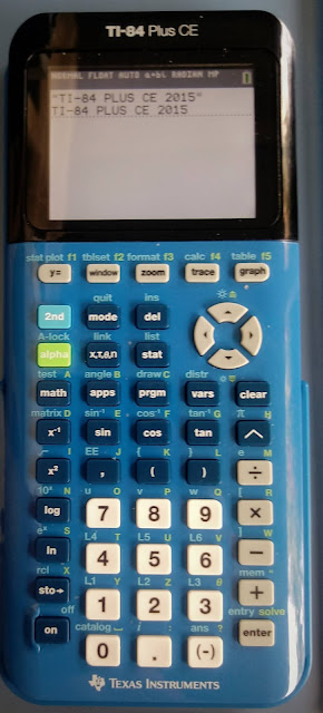
TI-84 Plus CE:  2015

TI-84 Plus CE Python Edition:  2021

Eddie

All original content copyright, © 2011-2021.  Edward Shore.   Unauthorized use and/or unauthorized distribution for commercial purposes without express and written permission from the author is strictly prohibited.  This blog entry may be distributed for noncommercial purposes, provided that full credit is given to the author. 

TI-86 and DM42/HP42S: Square Root Simplification

TI-86 and DM42/HP42S:  Square Root Simplification

Introduction

The program SQROOT attempts to factor √N into the form A√B (N, A, and B are positive integers).  The program tests whether X^2 evenly divides into N from X = 1 to int(√N).  If successful, let A = X and B = N/X^2.

Example:  

√88   (N = 88)

int(√88) = 9

Test:

88/9^2 ≈ 1.0864

88/8^2 = 1.375

88/7^2 ≈ 1.7959

88/6^2 ≈ 2.4444

88/5^2 = 3.52

88/4^4 = 5.5

88/3^2 ≈ 9.7778

88/2^2 = 22    

2^2 (4) divides into 88 evenly.  

Then A = 2, B = 22.  Therefore √88 = 2√22

TI-86 Program:  SQROOT

*  This code should work on the TI-83/TI-84 Plus family with no or very minor adjustments.

*  The arrow -> is made of two characters:  the minus sign (-) and the greater than sign (>).  

"2021-01-06 EWS"

Disp "√N -> A√B"

Prompt N

iPart(√N)→X

While X≠0

If fPart(N/X^2)==0

Then

X→A 

N/X^2→B

Goto A

Else

X-1→X 

End

End

Lbl A

Disp "√N = A√B : A=", A, "B=" , B

HP 42S/DM42/Free42 Program: SQROOT

*  The character ├ appends (attaches) alpha strings together.  To designate strings to be attached, press ENTER while in ALPHA entry mode.

*  Similarly, pressing RCL while ALPHA mode will allow you to recall the value of a register and attach it to current alpha string.

* The ALL mode is similar to the standard and float mode.

* Registers:  R00 = N, R01 = A, R02 = B

00 {52-Byte Prgm}

01 LBL "SQROOT"

02 "N?"

03 PROMPT

04 STO 00

05 SQRT

06 IP

07 STO 01

08 LBL 00

09 RCL 00

10 RCL 01

11 X↑2

12 ÷

13 STO 02

14 FP

15 X=0?

16 GTO 01

17 1

18 STO- 01

19 GTO 00

20 LBL 01

21 ALL

22 CLA

23 "√"

24 ARCL 00

25 ├"="

26 ARCL 01

27 ├"√"

28 ARCL 02

29 END

Examples

√88 = 2√22

√46 = 1√46

√178 = 1√178

√200 = 10√2

Eddie

All original content copyright, © 2011-2021.  Edward Shore.   Unauthorized use and/or unauthorized distribution for commercial purposes without express and written permission from the author is strictly prohibited.  This blog entry may be distributed for noncommercial purposes, provided that full credit is given to the author. 

HP Prime and TI-86: Minimum Vertical Curve Length

HP Prime and TI-86: Minimum Vertical Curve Length

Introduction

The program MVCL calculates the minimum vertical curve length for sight distances for crest curves (curve that rises then falls) and sag curves (curves that falls than rises). The equations used were determined by the AASHTO (American Association of Highway and Transportation Officials of Washington, D.C.).

HP Prime Program MVCL

EXPORT MVCL()
BEGIN
// Minimum stop speed
LOCAL g1,g2,a,c,l,s,g;

MSGBOX("Break = 2.5 s,
 Decel = 11.2 ft/s^2");

LOCAL l1:={15,20,25,30,35,40,45,
50,55,60,65,70,75,80};

LOCAL l2:={80,115,155,200,250,
305,360,425,495,570,645,730,
820,910};

INPUT({g1,g2,{c,l1}},"MVCL",
{"Grade1%:","Grade2%:",
"Speed:"});

s:=l2(c);
a:=ABS(g1-g2);

l:=2*s-2158/a;
IF s < l
l:=a*s^2/2158;
END;

g:=2*s-(400+3.5*s)/a;
IF s < g
g:=(a*s^2)/(400+3.5*s);
END;

PRINT();
PRINT("Stop speed (ft)");
PRINT("Crest curve: "+l);
PRINT("Sag curve: "+g);


END;

TI-86 Program MVCL

(744 bytes)

Input “GRADE %1:”, G1

Input “GRADE %2:”, G2

abs(G2-G1) → A

Disp “Break time = 2.5s”, “Decl. = 11.2 ft/s²”,

“Car Speed?”,”(mph)”

Menu(1,”15”,A,2,”20”,B,

3,”25”,C,4,”30”,D,

5,”35”,E,6,”40”,F,

7,”45”,G,8,”50”,H,

9,”55”,I,10,”60”,J,

11,”65”,K,12,”70”,L,

13,”75”,M,14,”80”,N)

Lbl A : 80 → S : Goto Z

Lbl B : 115 → S : Goto Z

Lbl C : 155 → S : Goto Z

Lbl D : 200 → S : Goto Z

Lbl E : 250 → S : Goto Z

Lbl F : 305 → S : Goto Z

Lbl G : 360 → S : Goto Z

Lbl H : 425 → S : Goto Z

Lbl I : 495 → S : Goto Z

Lbl J : 570 → S : Goto Z

Lbl K : 645 → S : Goto Z

Lbl L : 730 → S : Goto Z

Lbl M : 820 → S : Goto Z

Lbl N : 910 → S : Goto Z

Lbl Z

Disp “Stop speed (ft)”, “crest curve:”

2 * S – 2158 / A → L

If S > L

Then

Disp L

Else

A * S² / 2158 → L

Disp L

End

Disp “sag curve:”

2 * S – (400 + 3.5 * S) / A → G

If S > G

Then

Disp G

Else

(A * S²) / (400 + 3.5 * S) → G

Disp G

End

Examples:

Example 1:

Grade 1: -1.75%

Grade 2: 2.25%

Design Speed: 40 mph

Result:

Minimum Vertical Curve Length

Crest Curve: 70.5 ft

Sag Curve: 243.125 ft

Example 2:

Grade 1: -1%

Grade 2: 1.7%

Design Speed: 50 mph

Result:

Minimum Vertical Curve Length

Crest Curve: 50.740740741 ft

Sag Curve: 150.925925926 ft

Source:

Michael R. Lindberg, PE “Civil Engineering Reference Manual for the PE Exam” 11^th Ed. Professional Publications, Inc: Belmont, CA. 2008. ISBN 13-978-1-59126-192-2

Eddie

All original content copyright, © 2011-2019. Edward Shore. Unauthorized use and/or unauthorized distribution for commercial purposes without express and written permission from the author is strictly prohibited. This blog entry may be distributed for noncommercial purposes, provided that full credit is given to the author.

TI-86: Sequence Graphing

TI-86: Sequence Graphing

The program Sequen86 plots one recursive sequence with one initial condition. The function is stored in variable y1, with x presenting y1(n-1). The initial condition is assumed to be y1(1).

This program was originally posted on ticalc.org on April 28, 2001. Link: https://www.ticalc.org/archives/files/fileinfo/186/18667.html

18 years, wow, how time flies.

TI-86 Program Sequen86

(354 bytes)

Func

FnOff

PlOff

ClLCD

DelVar(L1)

DelVar(L2)

Outpt(6,1,”Let y1 = u”)

Outpt(7,1,”Let x = n-1”)

InpSt “y1 =”, Y

St>Eq(Y,y1)

Input “Initial Cond: “,I

Input “# of Steps: “,S

{I} → U

For(N, dimL U+1, S+1, 1)

y1(U(N-1)) → U(N)

End

seq(x,x,1,S+1) → L1

U → L2

0 → xMin

S+1 → xMax

min(U) – 1 → yMin

max(U) + 1 → yMax

Plot1(1,L1,L2)

FnOff 1

Disp “L1 = n”

Pause “L2 = u”

DispG

Example:

u(n) = u(n-1)/3 + 1/4

Initial condition, u(1) = 1/5

Number of Steps: 10

Set up for Sequen86:

y1 = x/3 + 1/4

The 2019 Version

Here is an alternate version, SEQGRAPH. Use U for U(n-1) and N for n. The program allows the initial condition for any value of N.

TI-86 Program SEQGRAPH

(277 bytes)

InpSt “U1(U,N) = “,S1

St>Eq(S1,U1)

Input “N Start = “,N

Input “U0 = “,U

Input “Steps: “,S

S + 1 → dimL xList

S + 1 → dimL yList

N → xList(1)

U → yList(1)

For(I, 2, S+1)

xList(I-1) + 1 → N

N → xList(I)

yList(I-1) → U

U1 → yList(I)

End

FnOff

PlOff

PlOn 1

Plot1(1,xList,yList)

ZData

Example:

u(n) = u(n-1)/3 + 1/4

Initial condition, u(1) = 1/5

Number of Steps: 10

Set up for SEQGRAPH:

U1 = U/3 + 1/4

N Start: 1

U0 = 1/5 (initial condition)

Eddie

All original content copyright, © 2011-2019. Edward Shore. Unauthorized use and/or unauthorized distribution for commercial purposes without express and written permission from the author is strictly prohibited. This blog entry may be distributed for noncommercial purposes, provided that full credit is given to the author.

TI-86: Angle Between Vectors, Vandermonde Matrix, Least Squares Algorithm, Chebyshev Polynomials (1st Kind)

TI-86: Angle Between Vectors, Vandermonde Matrix, Least Squares Algorithm, Chebyshev Polynomials (1^st Kind)

The TI-86 has one of the best interfaces for a graphing calculator I ever had the joy to work with. The TI-86 is an update of the TI-85. Here are some programs for the TI-86.

Angle Between Vectors

The program vangle calculates the angle between two angles. The angle is calculated in degrees.

TI-86 Program vangle

(75 bytes)

Prompt V1

Prompt V2

Disp cos⁻¹ (dot(V1,V2)/(norm V1*V2))

Example: [2, -3, 4] and [8, 1, -2]

Angle: 83.5823268926°

Vandermonde Matrix

The program vander creates a matrix based on a list of coefficients.

Example: {x, y, z} produces the matrix

[ [x^0, x^1, x^2], [y^0, y^1, y^2], [z^0, z^1, z^2] ]

TI-86 Program vander

(125 bytes)

Input “List: “, L1

dimL L1 → N

{N, N} → dimL MA

For(R, 1, N)

For(C, 1, N)

L1(R)^(C-1) → MA(R,C)

End

End

Disp “MA=”

Pause MA

Example: {2, 4, 7}

Result: [ [1, 2, 4], [1, 4, 16], [1, 7, 49] ]

Least Square Algorithm

The program LSQ taxes the matrices X and Y (Y is a one-column matrix), and calculates

(X^T X)^-1 (X^T Y).

LSQ is used to fit statistical fits with least squares.

TI-86 Program LSQ

(118 bytes)

Disp “Least Squares”

Input “Matrix X: “,MX

Input “Matrix Y: “,MY

(MX^T * MX)^-1 * (MX^T * MY) → ML

Disp “ML= “

Pause ML

Example:

MX = [ [1, 3, 2.0], [1, 4, 2.3], [1, 5, 2.6], [1, 8, 2.9] ]

MY = [ [1.6], [1.8], [2.1], [2.3] ]

Results:

ML = [ [-0.14444444449], [-1.666666667E-2], [0.88888888889] ]

Chebyshev Polynomials (1^st Kind)

The program tcheby calculates the numerical value of the Chebyshev polynomials of the 1^st Kind given its point, X, and the order, N.

TI-86 Program tcheby

(127 bytes)

Prompt X,N

If X>1 : Goto A

If X<-1 :="" b="" goto="" span="">

cos(N * cos⁻¹ X) → A

Goto C

Lbl A

cosh(N * cosh⁻¹ X) → A

Goto C

Lbl B

(-1)^N * cosh(N * cosh⁻¹ X) → A

Lbl C

Disp A

Example:

X = -2.5, N = 4, Result: 263.5

X = 0.5, N = 4, Result: -0.5

X = 2.5, N = 4, Result: 263.5

Eddie

All original content copyright, © 2011-2019. Edward Shore. Unauthorized use and/or unauthorized distribution for commercial purposes without express and written permission from the author is strictly prohibited. This blog entry may be distributed for noncommercial purposes, provided that full credit is given to the author.