HP Prime: Edge Diffraction Parametric Plot

HP Prime:  Edge Diffraction Parametric Plot

Introduction

The program EDGEDIFFRAC plots the complex amplitude of edge diffraction.  The equation is:

φp = φ0 / √2 * ( CS(t) + 1/2 * (1 + i) )

where:

φp = complex amplitude 

φ0 = unobstructed amplitude, can be a complex number

CS(t) = Cornu Spiral, defined as CS(t) = C(t) + i * S(t)

Cosine Fresnel Integral

C(t) = ∫( cos (π * s^2 / 2) ds for s = 0 to t)

Sine Fresnel Integral

S(t) = ∫( sin (π * s^2 / 2) ds for s = 0 to t)

i = √-1

HP Prime Program:   EDGEDIFFRAC

Notes:

1.  This program runs in the Parametric app.

2.  To allow for the program to be run from any app, the STARTAPP command is placed in the beginning of the program.

3.  To allow editing in any app, the Parametric. prefix is added to the variables Tmin, Tmax, and Tstep.   

4.  The QUOTE command is used to store functions to the graphing variables X1 and Y1.  

5.  The program runs faster in the emulator than the hardware calculator.  

6.  x1(t) is the real part of φp, and y1(t) is the imaginary part of φp. 

Code:

EXPORT EDGEDIFFRAC()

BEGIN

// Edge Diffraction 

// 2023-02-19 EWS

STARTAPP("Parametric");

// set radians mode

HAngle:=0;

// local variables

LOCAL ch,l,lc,pc;

LOCAL y,λ,z,w,φp;

 

// plot application

INPUT(Z0,"Unobstructed Amplitude",

"φ0:");

CHOOSE(l,"Change Color","Red","Indigo",

"Blue","Orange","Green");

lc:={#FF0000h,#400080h,#FFh,

#FFA500h,#C000h};

X1(COLOR):=lc[l];

Parametric.Tmin:=-5;

Parametric.Tmax:=5;

Parametric.Tstep:=0.25;

A:=RE(Z0);

B:=IM(Z0);

X1:=QUOTE(A/√2*(∫(COS(π*S^2/2),S,0,T)+1/2)

-B/√2*(∫(SIN(π*S^2/2),S,0,T)+1/2));

Y1:=QUOTE(A/√2*(∫(SIN(π*S^2/2),S,0,T)+1/2)

+B/√2*(∫(COS(π*S^2/2),S,0,T)+1/2));

CHECK(1);

STARTVIEW(10);

END;

Examples

Example 1:   φ0 =  2 + 6i

Example 2:  φ0 = 2.29

Source

Woan, Graham.  The Cambridge Handbook of Physics Formulas.  Cambridge University Press:  Cambridge, New York.   2003

All original content copyright, © 2011-2023.  Edward Shore.   Unauthorized use and/or unauthorized distribution for commercial purposes without express and written permission from the author is strictly prohibited.  This blog entry may be distributed for noncommercial purposes, provided that full credit is given to the author. 

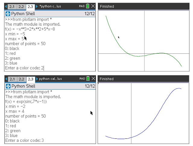
Python - Lambda Week: Plotting Functions

Python - Lambda Week: Plotting Functions

Welcome to Python Week!  This we we're going to cover calculus and the keyword lambda.

Note:  All Python scripts presented this week were created using a TI-NSpire CX II CAS.   As of June 2022, the lambda keyword is available on all calculators (in the United States) that have Python.   If you are not sure, please check your calculator manual. 

Plotting Functions

We can use the line:

f=eval("lambda x:"+input("f(x) = "))

for multiple applications.   Remember, lambda functions are not defined so that they can be used outside of the Python script it belongs to but it lambda functions are super useful!

This code is specific to the Texas Instruments calculators (TI-Nspire CX II (CAS), TI-84 Plus CE Python, TI-83 CE Premium Python Edition, but NOT the TI-82 Advanced Python).    For other calculators, HP Prime, Casio fx-CG 50, Casio fx-9750GIII/9860GIII, Numworks, or computer Python, apply similar language. 

plotlam.py:  Plotting with Lambda

from math import *

import ti_plotlib as plt

# this is for the TI calcs

# other calculators will use their own plot syntax

print("The math module is imported.")

# input defaults to string

# use the plus sign to combine strings

f=eval("lambda x:"+input("f(x) = "))

# set up parameters

x0=eval(input("x min = "))

x1=eval(input("x max = "))

# we want n to be an integer

n=int(input("number of points = "))

# calculate step size

h=(x1-x0)/n

# calculate plot lists

x=[]

y=[]

i=x0

while i<=x1:

  x.append(i)

  y.append(f(i))

  i+=h

# choose color (not for Casio fx-9750/9850GIII)

# colors are defined using tuples

colors=((0,0,0),(255,0,0),(0,128,0),(0,0,255))

print("0: black \n1: red \n2: green \n3: blue")

c=int(input("Enter a color code: "))

# plot f(x)

# auto setup to x and y lists

plt.auto_window(x,y)

# plot axes

plt.color(128,128,128)

plt.axes("axes")

# plot the function

plt.color(colors[c])

plt.plot(x,y,".")

plt.show_plot()

All original content copyright, © 2011-2022.  Edward Shore.   Unauthorized use and/or unauthorized distribution for commercial purposes without express and written permission from the author is strictly prohibited.  This blog entry may be distributed for noncommercial purposes, provided that full credit is given to the author. 

TI-84 Plus CE, TI-Basic and Python: Dynamic and Goal Average

TI-84 Plus CE, TI-Basic and Python:  Dynamic and Goal Average 

Dynamic Average

The dynamic average is defined as:

Σx_i / m   from i = 1 to m, m ≤ n

A new list is created:

1st point has the value of the first data value,

2nd point has the value of the first two data values, 

3rd point has the value of the first three data values,

...

nth point is the arithmetic average of the entire list.

The TI-Basic Version plots the averages in a stat plot, while the Python version returns a list.

Remember:  In TI-Basic, the pointer starts at 1, while with Python, the pointer starts at 0.  Also, my Python programs will require you to enter the number of data points in advance. 

TI-84 Plus CE TI-Basic Program:  DYNAVG

"EWS 2022-04-18"

Input "DATA? ", L1   // [ 2nd ] [ 1 ]

seq(X,X,1,dim(L1),1)→L2   // [ 2nd ] [ 2 ]

cumSum(L1)/L2→L3   // [ 2nd ] [ 3 ]

Func: FnOff : PlotsOff

Plot1(Scatter,L2,L3)

ZoomStat

TI-84 Plus CE Python File: dynavg.py

# 2022-04-20 EWS

d=eval(input("# points? "))

x=[ ]

s=[ ]

a=[ ]

for i in range(d):

  w=eval(input("point "+str(i+1)+"? "))

  x.append(w)

  t=sum(x)

  s.append(t)

  v=t/(i+1)

  a.append(v)

print("cumulative sum:")

print(s)

print("dynamic average:")

print(a)

Example:

Input:  Data Points:  {4, 5.6, 3.9, 5.6, 5.7, 5.8, 7.2, 6.4}

Result: Dynamic Averages: {4, 4.8, 4.5, 4.775, 4.96, 5.1, 5.4, 5.525}

Goal Average

You have a goal, for example:  

*  reach a set number of steps

*  raise a set amount of revenue

*  score a set amount of points during a season of basketball

You have a set amount of times (days, months, years, etc.) (n) and you have a certain amount of data points (m).   Assuming you have time left in your program, what is the remaining amount needed and average per period left?  (This assumes that m < n).  

TI-84 Plus CE TI-Basic Program:  GOALAVG

"2022-04-18 EWS"

Input "GOAL? ", T

Input "TIMES? ", n

Input "DATA? ", L1

sum(L1)→S

dim(L1)→M

If S≥T

Then

Disp "GOAL MADE"

Else

T-S→D

D/(N-M)→A

Disp "TO GO =",D

Disp "AVG =",A

End

TI-84 Plus CE Python File: goalavg.py

# 2022-04-20 EWS

t=eval(input("Goal? "))

n=eval(input("# times? "))

m=eval(input("# data points? "))

s=0

x=[ ] 

for i in range(m):

  w=eval(input("point "+str(i+1)+"? "))

  x.append(w)

  s+=w

if s>=t:

  print("Goal made!")

else:

  d=t-s

  a=d/(n-m)

  print("To go: "+str(d))

  print("Average: "+str(a))

Example:

Input:  

Goal:  100,000

# Times:  14  (n)

# Data Points: 6  (m)

Data:  {5466, 8316, 8821, 9340, 6726, 8011}

Results:

To Go:  53539

Average:  6692.375

Eddie

All original content copyright, © 2011-2022.  Edward Shore.   Unauthorized use and/or unauthorized distribution for commercial purposes without express and written permission from the author is strictly prohibited.  This blog entry may be distributed for noncommercial purposes, provided that full credit is given to the author. 

7000G Retro Month - June 12 Edition

7000G Retro Month - June 12 Edition

Introduction

Welcome to the 7000G Retro Month, which features programming for the classic Casio calculators from the mid/late 1980s:  primarily fx-7000G and fx-7500G.  Since the programming language stays similar throughout the years, programs can be translated to the fx-6300G and later graphing calculators with little to no adjustments.  Non graphic programs should be ported to the fx-4000P, fx-4500P (A), fx-3650p (II), fx-50F Plus (II), and fx-5800P with little to no adjustments.  

7000G Retro Month takes place every Saturday during June 2021.

To make text easier to type, I can going to use the following text friendly symbols for the following:

->  for →

/I for ⊿

=> for ⇒

What do you think?   Unicode or simple text equivalents?  

- - - - - - -- - -- - -

Today's subject revolves around Graphics.  Enjoy!

- - - -- - - -- - -- -- -

Get a emulator or graphing calculator to see the results.

Quadratic Fit by Two Roots

Given two roots A and B, the program generates a quadratic equation and it's graph.   The program assumes that the vertex is a minimum.

Y = (X - A) (X - B)

"ROOT1" -> A

"ROOT2" -> B

"Y = X^2 - " /I

A+B /I

"X + " /I

AB /I

Cls

Graph Y=(X-A)(X-B)

Polar Plotting (Self Contained)

I usually use Radians (Mode 5 for fx-7000G, fx-7500G, fx-6300G) angle mode when it comes to graphics and calculus.  To set/change each equation, you will need to edit the program here.  I state the equation to be in the form r(T) where T = θ.  

On the Rec command, x is stored to I and y is stored to J.  (specific to fx-7000G, fx-7500G, fx-6300G)

"POLAR R(T)"

Rad

"RMIN"? -> A

"RMAX"? -> B

"N"? -> N

(B-A)÷N -> H

A-H -> T

Cls

Lbl 1

T+H -> T

[insert r(T) here]

Rec(Ans, T)

Plot I,J

T<B => Goto 1

Cubic Bezier Curve

This program plots a cubic Bezier curve with the following variables:

(x0, y0):  A = A[0], B = A[1]  (exact fit)

(x1, y1):  C = A[2], D = A[3]

(x2, y2):  E = A[4], F = A[5]

(x3, y3):  G = A[6], H = A[7]   (exact fit)

Cls

0 -> I

"CUBIC BEZIER"

Lbl 1

"X"? -> A[ I ]

Isz I

"Y"? -> A[ I ]

Isz I

I < 8 => Goto 1

0 -> T

Lbl 2

A(1-T)^3 + 3C(1-T)^2 T + 3E(1-T) T^2 + GT^3 -> X

B(1-T)^3 + 3D(1-T)^2 T + 3F(1-T) T^2 + HT^3 -> Y

Plot X,Y

T+.02 -> T

T<1 => Goto 2

Press [ G<>T ] to see the graph.  

Polygon Drawing

The programs allow the user to draw many lines in a row by connecting points.   The original point are stored in variables E and F.   To complete the polygon, use (E, F) as the final point.  

The prompt MORE:  enter 0 to stop, anything else to continue connecting points

Cls

"X0"? -> A : A -> E

"Y0"? -> B : B -> F

Plot A,B

Lbl 1

"ORIG (E,F)"

"NEXT X"? -> C

"NEXT Y"? -> D

0 -> T

Lbl 2

(1-T)A+CT -> X

(1-T)B+DT -> Y

Plot X,Y

T+.02->T

T<1 => Goto 2

C -> A : D -> B

"MORE"? -> M

M≠0 => Goto 1

Drawing an Ellipse

This program draws an ellipse.  

"ELLIPSE"

"X RADIUS"? -> A

"Y RADIUS"? -> B

Rad

Cls

Range -A-.5,A+.5,(2A+1)÷20,-B-.5,B+.5,(2B+1)÷20

0 -> T

Lbl 1

Plot A cos T, B sin T

T+2π÷64 -> T

T<2π => Goto 1

Press [ G<>T ] to see the graph.  

Eddie

All original content copyright, © 2011-2021.  Edward Shore.   Unauthorized use and/or unauthorized distribution for commercial purposes without express and written permission from the author is strictly prohibited.  This blog entry may be distributed for noncommercial purposes, provided that full credit is given to the author. 

RPL Programming Tutorial - Part 5 - HP 49g+/50g: Prompt and Introduction to Algebraic Objects

Excuse me, but I must prompt you for something.

Welcome to the second week of my RPL tutorials, using the Hewlett Packard HP 49g+ and 50g calculators. Today's session will cover the PROMPT command.

The PROMPT command sets the program to ask the user for input. That input can be whatever you practically want: text, numbers, matrices, and equations. The user enters the requested information and presses the key sequence [LS] [ON] (CONT) . The [LS] [ON] sequence tells the calculator that the user is ready to move on.

The PROMPT structure is this:

"String that asks the user for input" PROMPT

Today we will do two programs using PROMPT: a simple program that picks an integer from 1 to N, and a more complex one that takes an equation and graphs it.

In this bag we have lotto balls from 1 to 49, and the first number is...

This program will ask you for a number (N), the number of draws (X), and the calculator will return X integers randomly selected from 1 to N. One caveat in this program is that the numbers selected can repeat.

The Program ONETO

Comments will be italicized, starting with an asterisk. You will not need to pre-load the stack with ONETO - all the inputs will be prompted for.

As a reminder:

[LS] means the left shift key (white on the 50g, green on the 49g+)
[RS] means the right shift key (orange on the 50g, red on the 49g+)
Pressing [ALPHA] twice will put the calculator in ALPHA-LOCK mode. If you want lower case letters, press [LS] then the letter. For greek and other characters, select [RS] then the letter.

Hint:

During program entry, you can press [RS] [ . ] for a carriage return. This can make program entry easier to see and read. Best of all, this does not affect program entry or execution.

Note:

The key [big X] is located on the 5th rows of keys up from the bottom. I will use this to distinguish the X character from the times key [ x ].

Program Input:

[RS] [ + ] ( << >> )
* Start the program entry
[RS] [ x ] ( "" )
[ALPHA] [ALPHA] [MODE] (H) [TOOL] (I) [APPS] (G) [MODE] (H) [SPC] [EVAL] (N) [TAN] (U) [HIST] (M) [F2] (B) [F5] (E) [ √ ] (R) [RS] [+/-] (=) [ALPHA]
[ &rarr ] [LS] [EVAL] (PRG) [NXT] [F5] (IN) [NXT] [F1] (PROMPT)
* Enters the first prompt request, "HIGH NUMBER="
[RS] [ x ] ( "" )
[ALPHA] [ALPHA] [LS] 3 (#) [SPC] [ ' ] (O) [F6] (F) [SPC] [F4] (D) [ √ ] (R) [F1] (A) [+/-] (W) [SIN] (S) [RS] [+/-] (=) [ALPHA]
[ &rarr ] [F1] (PROMPT)
* Enters the second prompt request, "# OF TIMES="
[RS] 0 ( &rarr ) [ALPHA] [EVAL] (N) [SPC] [big X]
* Enters N and X and declares them as local variables
[RS] [ + ] (<< >>) 1 [SPC] [big X]
[F6] (PRG) [F3] (BRCH) [LS] [F4] (FOR)
* Use the current menu to go back to the Program level, enters FOR-NEXT structure
[ALPHA] [STO>] (K) [SPC] [ALPHA] [EVAL] (N)
[LS] [SYMB] (MTH) [NXT] [F1] (PROB) [F4] (RAND)
[ x ] 1 [ + ] [NXT] [F6] (MTH) [F5] (REAL) [NXT] [IP] (F5)
* Enters the commands for the For loop
[ENTER]
* Terminate program entry

[ ' ] [ALPHA] [ALPHA] [ ' ] (O) [EVAL] (N) [F5] (E) [COS] (T) [ ' ] (O) [ALPHA] [ENTER] [STO>]

The completed program:

<< "HIGH NUMBER=" PROMPT
"# OF DRAWS=" PROMPT
&rarr N X
<< 1 X
FOR K N RAND * 1 + IP
NEXT >> >>

Instructions:

1. Run ONETO
2. The calculator will prompt "HIGH NUMBER=" at the top of the screen. Enter the high number and then press [LS] [ON] (CONT).
3. The calculator will prompt "# OF DRAWS=" at the top of the screen. Enter the number of draws and then press [LS] [ON] (CONT).
4. The calculator fills the stack with randomly selected numbers. Use [HIST] and [ &uarr ] to view the numbers. Press [ON] when done viewing the stack.
5. You may want to clear the stack before continuing.

Example:

A possible set of 12 random integers from 1-12 is: 9, 4, 7, 2, 11, 1, 10, 4, 1, 4, 1, 7.

Graphing an equation from the Stack Program

This program graphs a given an function y(x) using specified window settings. This is just one way of graphing an equation, which is an alternate way to graphing functions without using the graphing set up screens (Y=, WIN, GRAPH, and 2D/3D). The function can be traced and analyzed just like any other functions that are plotted.

The Catalog

You can access all the commands that the 49g+ and 50g has in the catalog. To access the catalog, press [RS] [SYMB] (CAT). If you press [ALPHA] and a letter, you can quickly scroll to that part of the catalog. You may be able to get a few letters if you are fast enough.

The other thing that is nice about the 49g+ and 50g is that the commands can be typed. This may be a helpful and faster alternate than trying to hunt commands in the menu or catalog. However, in this tutorial, the keystrokes I show will make use of the catalog.

Commands that are Used

* XRNG: Sets the left and right boundaries of the plot screen. The left boundary is taken from Level 2; the right boundary is taken from Level 1.
* YRNG: Sets the bottom and top boundaries of the plot screen. The bottom boundary is taken from Level 2; the top boundary is taken from Level 1.
* FUNCTION: Sets the calculator to Function mode.
* STEQ (Store Equation): Stores an equation in the EQ variable. The EQ variable is a system variable which the calculator uses to plot and solve equations with. EQ can have a list of more than one equation or expression.
* INDEP: Sets a variable as independent. Useful when setting up a plot. It makes sense to make the independent variable 'X' or even 'T' or ' θ', but you can make the independent variable anything you want.
* ERASE: Erases the plot screen and gets the calculator ready to draw a fresh, new plot.
* DRAW: Has the calculator draws whatever is stored in EQ.
* DRAX (Draw the Axes): Has the calculator draw the axes.
* PICTURE: Switches the calculator to the plot (picture) environment.

With all these commands to play with, let's program GRPFX.

The Program GRPFX

[RS] [ + ] (<< >>)
[RS] [ x ] ( "" )
[ALPHA] [ALPHA] [1/x] (Y) [LS] [ - ] (parenthesis) [big X] [RS] [+/-] (=)
* Input the string "Y="
[LS] [EVAL] (PRG) [NXT] [F5] (IN) [NXT] [F1] (PROMPT)
* Inserts the Prompt command. Leave this menu open.
[RS] [SYMB] (CAT) [ALPHA] [SIN] (S) scroll until you find STEQ
[F6] (OK)
* Use the catalog to find the STEQ command. You can hold [ &darr ] and [ &uarr ] to quickly scroll the catalog.
[RS] [SYMB] (CAT) [ALPHA] [F6] (F) find FUNCTION [F6] (OK)
* Set the calculator to FUNCTION mode
[ ' ] [ (big) X ] [ &rarr ] [RS] [SYMB] [ALPHA] [TOOL] (I) find INDEP [F6] (OK)
* Set X to be the independent variable.
[RS] [ x ] ( "") [ALPHA] [ALPHA] [big X] [HIST] (M) [TOOL] (I) [EVAL] (N) [RS] [+/-] (=) [F1] (PROMPT)
[RS] [ x ] ( "" ) [ALPHA] [ALPHA] [big X] [HIST] (M) [F1] (A) [big X] [RS] [+/-] (=) [F1] (PROMPT)
[RS] [SYMB] (CAT) [big X] find XRNG [F6] (OK)
* Prompt for the left and right boundaries, then use the XRNG command.
[RS] [ x ] ( "" ) [ALPHA] [ALPHA] [1/X] (Y) [HIST] (M) [TOOL] (I) [EVAL] (N) [RS] [+/-] (=) [F1] (PROMPT)
[RS] [ x ] ( "" ) [ALPHA] [ALPHA] [1/X] (Y) [HIST] (M) [F1] (A) [big X] [RS] [+/-] (=) [F1] (PROMPT)
[RS] [SYMB] (CAT) [ALPHA] [1/X] (Y) find YRNG [F6] (OK)
* Prompt for the bottom and top boundaries, then use the YRNG command.
[RS] [SYMB] (CAT) [ALPHA] [F5] (E) find ERASE [F6] (OK)
[RS] [SYMB] (CAT) [ALPHA] [F4] (D) find DRAX [F6] (OK)
[RS] [SYMB] (CAT) [ALPHA] [F4] (D) find DRAW [F6] (OK)
* Input the ERASE, DRAX, and DRAW commands.
[RS] [SYMB] (CAT) [ALPHA] [SYMB] (P) find PICTURE [F6] (OK) [ENTER]
* Input the PICTURE command and terminate program entry.

The completed program:

<< "Y(X)=" PROMPT
STEQ
FUNCTION
'X' INDEP
"XMIN=" PROMPT "XMAX=" PROMPT XRNG
"YMIN=" PROMPT "YMAX=" PROMPT YRNG
ERASE DRAX DRAW
PICTURE >>

Algebraic Objects

Simply put, algebraic objects are equations or formulas that are enclosed in single quotes. Examples include:

'1'
'X+2/5'
'SIN(π-1/2)'
'e^5.2-SQ(3)'

Algebraic objects gives the user an alternative (and maybe easier) way for the user to enter equations. In Part 6, we will explore several common functions that can be used with algebraic objects.

We can also enter equations using the RPN method. Let's try an example:

To enter 'X^2 + 3X - 1', we can enter this two ways. Assume X does not have anything stored in it. Purge X if need be.

RPN Way: [big X] [ENTER]
* duplicates X.
[LS] [ √ ] (x^2) [LS] [ &rarr ] (SWAP) 3 [ x ] [ + ] 1 [ - ] [EVAL]

Use [EVAL] to simplify the expression.

Algebraic Object: [ ' ] [big X] [y^x] 2 [ + ] 3 [ x ] [big X] [ - ] 1 [ENTER]

Instructions for GRPFX:

1. Run GRPFX. All the input will be asked for you, so you don't need anything in the stack to start with.
2. At the "Y(X)=" prompt, enter a function in X. You can use RPN, an algebraic object, or use the equation writer. Please be aware that the prompt may disappear when you are entering the function, just continue. Press [LS] [ON] (CONT) to continue.
3. At the "XMIN=" prompt, enter the left boundary, then press [LS] [ON] (CONT).
4. At the "XMAX=" prompt, enter the right boundary, then press [LS] [ON] (CONT).
5. At the "YMIN=" prompt, enter the bottom boundary, then press [LS] [ON] (CONT).
6. At the "YMAX=" prompt, enter the top boundary, then press [LS] [ON] (CONT).
7. You will see the function plotted. Use [F3] [F2] to trace the function. [F4] will give you access to function analysis such as ROOT, SLOPE, and AREA. Press [ON] to get back to the home screen.

The following pictures show GRPHX in action while plotting y(x) = x^2 + 3x - 1. Using the window, X = [-10, 10] and Y = [-10, 10]. (I am took pictures at a coffee shop using the iPad)

Hope you enjoyed Part 5. Come back for Part 6 where we explore cool functions with algebraic objects.

This tutorial is property of Edward Shore. Mass reproduction or distribution requires express permission of the author.