HP 15C: Quadratic Regression

HP 15C:  Quadratic Regression

Setup, Normal Equations, and Registers Used

This program fits bivariate date (x,y) to the quadratic polynomial:

y = c + b * x + a * x^2

This program uses the matrix feature of the HP 15C.  

The normal equations that are solved are:

n * c + Σx * b + Σx^2 * a = Σy

Σx *c + Σx^2 * b + Σx^3 *a = Σxy

Σx^2 * c + Σx^3 * b + Σx^4 * a = Σ(x^2 y)

Matrix A = 

[ [ n, Σx, Σx^2 ]

[ Σx, Σx^2, Σx^3 ]

[ Σx^2, Σx^3, Σx^4 ] ]

Matrix B = 

[ [ Σy ]

[ Σxy ]

[ Σ(x^2 y) ] ]

Matrix C = (Matrix B)^-1 Matrix A

[ [ c ] 

[ b ] 

[ a ] ]

Registers Used:

R0:  x data point, row pointer

R1:  y data point, column pointer

Default Statistics Registers:

R2:  n

R3:  Σx

R4:  Σx^2

R5:  Σy

R6:  Σy^2

R7:  Σxy

Additional Statistics Registers:

R8:  Σx^3

R9:  Σx^4

R.0:  Σ(x^2 y)   ("register point zero":  press the decimal point before the 0)

Instructions

1.  Run label A to clear the matrices and registers.  This needs to be done in order to get the most accurate results.  Zero is displayed to indicate when the calculator is ready.  

2.  For each point, enter y data point, press [ ENTER ], x data point, and run label B.  The number of data points (n) will be displayed.  

3.  To calculate the coefficients, run label C.   The coefficients c, b, and a are displayed in order.

Matrix Operations Used

MATRIX 0:  clear all the matrices 

MATRIX 1:  sets the row and counter pointer to 1,1.   

User Mode Set:  automatically advances the pointer to the right row by row.   In programs, turning on and off User Mode is not a step.  However, storage and recall operations in User Mode are marked with a "u" after the step number.  Be careful because if a matrix's pointers (row in R0 and column in R1) return to (1,1), while in USER mode, the next program is skipped.  A special acknowledgement to Torsten for pointing this to me.  

HP 15C Program Code: Quadratic Regression 

Program Memory:  67 steps, 90 bytes

Needs 15 additional memory registers to store the three matrices.

Comments begin with a hash symbol.  #

#  Label A:   Initialization

001 :  42,21,11 :   LBL A

002 :  42,34 :  CLEAR REG

003 :  42,16, 0 :  MATRIX 0

004 :  0 :   0

005 :  43,32  : RTN

# Label B:  Data Entry and Processing

006 : 42,21,12 :  LBL B

007 : 44, 0 :   STO 0

008 :  43,11 : x^2

009 :  34  :  x<>y

010 :  44, 1  : STO 1

011 :  20  :  ×

012 :  44,40,.0 :  STO+ .0  (# store-add to register point zero)

013 :  45, 0  : RCL 0  

014 :  3 :  3

015 :  14 : y^x

016 :  44,40, 8 :  STO+ 8

017 :  45,20, 0 :  RCL× 0

018 :  44,40, 9 : STO+ 9

019 :  45, 1 : RCL 1

020 :  45, 0 : RCL 0

021 :  49  : Σ+

022 :  43,32 : RTN

# Label C:  Calculation

023 : 42,21,13 : LBL C

024 : 3 :  3

025 : 36 : ENTER

026 : 42,23,11 : DIM A

027 : 42,16, 1 : MATRIX A

# Matrix A - Row 1

# Turn on USER Mode ( [ f ] [ RCL ] (USER))

028 : 45, 2 : RCL 2

029 u 44,11 :  STO A

030 : 45, 3 : RCL 3

031 u 44,11 : STO A

032 :  45, 4 :  RCL 4

033 u 44,11 : STO A

# Matrix A - Row 2

034 : 45, 3 : RCL 3

035 u 44,11 : STO A

036 : 45, 4 :  RCL 4

037 u 44,11 : STO A

038 :  45, 8 : RCL 8

039 u 44,11 : STO A

# Matrix A - Row 3

040 : 45, 4 : RCL 4

041 u 44,11 : STO A

042 : 45, 8:  RCL 8

043 u 44,11 : STO A

044 : 45, 9 : RCL 9

045 u 44,11 : STO A

# Turn off USER Mode (unless the next step would be skipped unnecessarily)

# Matrix B

046 : 42,16, 1 : MATRIX 1

047 : 3 :  3

048 : 36 : ENTER

049 : 1 : 1

# Turn on USER Mode

050 : 42,23,12 : DIM B

051 : 45, 5 : RCL 5

052 u 44,12 : STO B

053 : 45, 7 : RCL 7

054 u 44,12 : STO B

055 : 45,.0 : RCL .0   (# recall registers point-zero)

# Turn off USER Mode (unless the next step would be skipped unnecessarily and in this case, an Error 11 would occur)

056 :  44,12 : STO B

# Matrix C - Results

057 : 42,26,13 : RESULT C

058 : 45,16,12 : RCL MATRIX B

059 : 45,16,11 : RCL MATRIX A

060 : 10 : ÷

061 : 42,16, 1 : MATRIX 1

062 u 45,13 : RCL C

063 : 31 : R/S

064 u 45,13 : RCL C

065 : 31 : R/S

066 u 45,13 : RCL C

067 : 43,32 : RTN

Examples

Example 1:

(3, 1.3)

(4, 1.6)

(5, 1.5)

(6, 1.4)

c = -0.54

b = 0.92

a = -0.1

y = -0.54 + 0.92 x - 0.1 x^2

Example 2:

(0, 99.856)

(3, 97.232)

(5, 93.481)

(7, 96.005)

(10, 102.008)

c ≈ 100.3437

b ≈ -2.5318

a ≈ 0.2495

y ≈ 100.3437 - 2.5318 x + 0.2495 x^2

Enjoy!

Eddie

All original content copyright, © 2011-2023.  Edward Shore.   Unauthorized use and/or unauthorized distribution for commercial purposes without express and written permission from the author is strictly prohibited.  This blog entry may be distributed for noncommercial purposes, provided that full credit is given to the author. 

TI 84 Plus CE: Cauchy Fit Regression

TI 84 Plus CE: Cauchy Fit Regression

Note, in this blog capital and lower case letter variables are not assumed to be the same,  hence A ≠ a, B ≠ b, C ≠ c.

Derivation

General Equation:

Y = 1 / (A * (x + B)^2 + C)

We can set the equation in a general quadratic equation format by:

Y = 1 / (A * (x + B)^2 + C)
1/Y = A * (x + B)^2 + C
1/Y = A * (x^2 + 2*B*x + B^2) + C
1/Y = A*x^2 + 2*A*B*x + A*B^2 + C
1/Y = A*x^2 + 2*A*B*x + [A*B^2 + C]

Let:
y = 1/Y
a = A
b = 2*A*B
c = A*B^2 + C

Then:
y = a*x^2 + b*x + c

This form can be used when using a graphing or scientific calculator to calculate quadratic regression. 

We can solve for A, B, C:

A = a

b = 2*A*B
B = b / (2*A)

c = A*B^2 + C
C = c - A*B^2

To find a Cauchy regression fit:

1.  Enter the x data.
2.  Enter the y data but take the reciprocal of each y data point. 
3.  Run the Quadratic Regression:  y = a*x^2 + b*x + c
4.  Solve for the Cauchy regression to get the coefficients:

A = a
B = b / (2*A)
C = c - A*B^2

TI-84 Plus CE Program:  CAUCHFIT
Size:  200 Bytes

"2020-07-31 EWS"
Disp "CAUCHY FIT"
Input "X DATA? ", L1
Input "Y DATA? ", L3
1 / L3 → L2
QuadReg L1, L2
a → A
b / (2 A) → B
c - A B^2 → C
ClrHome
Output(3,1,"Y=1/(A(X+B)^2+C)"
Output(4,1,"A=")
Output(4,3,A)
Output(5,1,"B=")
Output(5,3,B)
Output(6,1,"C=")
Output(6,3,C)
Pause

Notes:

1.  The variables a, b, and c are from the VARS, Statistics, EQ menu.

2.  x data is stored in L1, 1/y data is stored in L2, and y data is stored in L3.  To call lists L1, L2, and L3, press [ 2nd ] [ 1 ], [ 2nd ] [ 2 ], and [ 2nd ] [ 3 ], respectively. 

3.  The use of Output should allow this code to be programmed on earlier TI-83 Plus and TI-84 Plus calculators. 

Example

X = { 1, 1.5, 2, 2.5 , 3}
Y = { 0.0774, 0.0577, 0.0442, 0.0347, 0.0278}

Results:

A = 1.823972632
B = 1.157397925
C = 4.437539736

y ≈ 1 / ( 1.823972632 * (x + 1.157397925)^2 + 4.437539736 )

Source:

Kolb, William M.  Curve Fitting For Programmable Calculators IMTEC.  Bowie, MD 20716.  1982.  ISBN-10:  0-943494-00-01


Stay safe and sane everyone.  Blessings,

Eddie

All original content copyright, © 2011-2020.  Edward Shore.   Unauthorized use and/or unauthorized distribution for commercial purposes without express and written permission from the author is strictly prohibited.  This blog entry may be distributed for noncommercial purposes, provided that full credit is given to the author.

R Programming Demo

R Programming Demo

This is a short demonstration of various things in R, some from an online class I recently completed and some from learning about R in its manual.   

Matrix Multiplication

> "Matrix Multiplication"

[1] "Matrix Multiplication"

> a<-matrix(c(1,3,4,-8),nrow=2,byrow=TRUE)

> a

     [,1] [,2]

[1,]    1    3

[2,]    4   -8

> b<-matrix(c(-3,2,0,1),nrow=2,byrow=TRUE)

> b

     [,1] [,2]

[1,]   -3    2

[2,]    0    1

> "Element by Element"

[1] "Element by Element"

> a*b

     [,1] [,2]

[1,]   -3    6

[2,]    0   -8

> "Linear Algebra Multiplication: Use %*%"

[1] "Linear Algebra Multiplication: Use %*%"

> a%*%b

     [,1] [,2]

[1,]   -3    5

[2,]  -12    0

Solving a Linear Equation

> "Solving a Linear System"

[1] "Solving a Linear System"

> A <- matrix(c(3,5,-5,-1,0,3,13,4,-3),nrow=3,byrow=TRUE)

> A

     [,1] [,2] [,3]

[1,]    3    5   -5

[2,]   -1    0    3

[3,]   13    4   -3

> x <- matrix(c(11,-2,10),nrow=3)

> x

     [,1]

[1,]   11

[2,]   -2

[3,]   10

> solve(A,x)

           [,1]

[1,]  0.1707317

[2,]  1.4878049

[3,] -0.6097561

Selecting Elements from a Vector

> "Selecting Things from a List"

[1] "Selecting Things from a List"

> randomvect <- c(-1.597,3.638,0.055,2.606,-2.053,-4.565,-2.470,-2.990,3.002,0.747,-2.813,2.524,0.096,-4.409,0.637)

> randomvect

 [1] -1.597  3.638  0.055  2.606 -2.053 -4.565 -2.470 -2.990  3.002  0.747 -2.813  2.524  0.096 -4.409  0.637

> "Select Every Third Element"

[1] "Select Every Third Element"

> randomvect[c(FALSE,FALSE,TRUE)]

[1]  0.055 -4.565  3.002  2.524  0.637

> "Select Elements Greater Than Zero"

[1] "Select Elements Greater Than Zero"

> randomvect[randomvect>0]

[1] 3.638 0.055 2.606 3.002 0.747 2.524 0.096 0.637

> "Select Elements In Between -1 and 1"

[1] "Select Elements In Between -1 and 1"

> randomvect[randomvect>-1 & randomvect<1]

[1] 0.055 0.747 0.096 0.637

Basic Linear Fit

> xdata <- c(-2,-1,-0,1,2,3,4)

> ydata <- c(-0.56,-0.36,0.15,0.33,0.52,0.77,0.93)

> df <- data.frame(x = xdata, y = ydata)

> df

   x     y

1 -2 -0.56

2 -1 -0.36

3  0  0.15

4  1  0.33

5  2  0.52

6  3  0.77

7  4  0.93

> fit<-lm(df$y~df$x)

> fit

Call:

lm(formula = df$y ~ df$x)

Coefficients:

(Intercept)         df$x 

  0.0007143    0.2535714 

> "Clear the Plot Screen"

[1] "Clear the Plot Screen"

> plot.new()

> "Scatterplot"

[1] "Scatterplot"

> plot(df$x,df$y,xlab="x",ylab="y",main="Demo Scatterplot")

> "Linear Plot"

[1] "Linear Plot"

> abline(lm(df$y~df$x),col="blue",lw=2)

Plot the Trigonometric Numbers

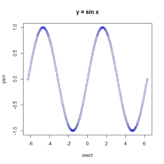
> "Plot The Trig Functions"

[1] "Plot The Trig Functions"

> xvect <- seq(-2*pi,2*pi,by=pi/64)

> ysin <- sin(xvect)

> plot.new()

> plot(xvect,ysin,main="y = sin x",col="blue")

> xtan <- seq(-pi/4, pi/4, by = pi/64)

> ytan <- tan(xtan)

> par(mfrow=c(2,2))

> plot(xvect, ysin, main = "y = sin x", xlab="x", ylab="y", col="blue",pch=8)

> plot(xvect, ycos, main = "y = cos x", xlab="x", ylab="y", col="red", pch=16)

> plot(xtan, ytan, main = "y = tan x", xlab="x", ylab="y", col="forestgreen", pch=20)

Quadratic Fit

> "Quadratic Fit"

[1] "Quadratic Fit"

> x <- c(-3.5,-2.25,-1.15,0,1.15,2.25,3.5)

> y <- c(10.6,6.3,3.1,2,3.3,6.4,10.4)

> plot(x,y,main="Quadratic Fit",col="chocolate",pch=20)

> fit <- lm(y~x+I(x^2))

> cvect <- coef(fit)

> xrng <- seq(-3.5,3.5,by=.01)

> yrng <- cvect[1] + cvect[2]*xrng + cvect[3]*xrng^2

> lines(xrng,yrng)

Histogram and One Variable Statistics

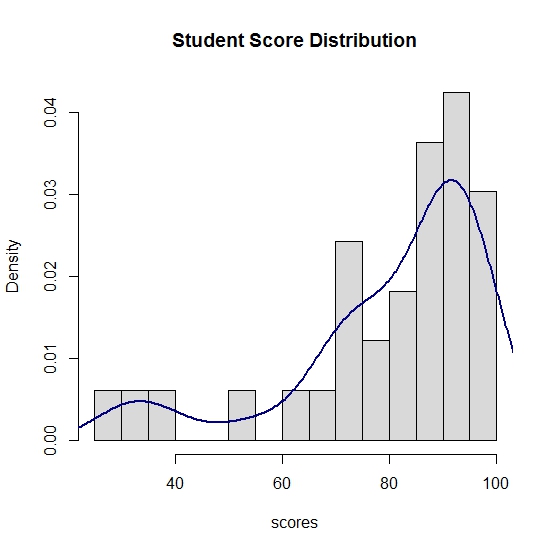
> scores <- c(99,97,96,95,94,29,39,90,92,92,91,86,84,54,65,72,76,77,81,82,90,33,93,92,89,88,90,98,68,71,73,75,97)

> "Minimum Score"

[1] "Minimum Score"

> min(scores)

[1] 29

> "Maximum Score"

[1] "Maximum Score"

> max(scores)

[1] 99

> "Average Score"

[1] "Average Score"

> mean(scores)

[1] 80.24242

> "Number of Students"

[1] "Number of Students"

> length(scores)

[1] 33

[1] "Basic Histogram"

> hist(scores)

> "10 Categories and Labels"

[1] "10 Categories and Labels"

> hist(scores, breaks=10, main="Student Score Breakdown", col="yellow")

> "Fiting a Distribution"

[1] "Fiting a Distribution"

> hist(scores, breaks=10, main="Student Score Distribution", col="gray85",prob=TRUE)

> lines(density(scores), lwd=2, col="navy")

Citation:

  R Core Team (2015). R: A language and environment for statistical computing. R Foundation for Statistical Computing, Vienna, Austria. URL

  http://www.R-project.org/.

A personal note, thank you for your support.  My mom and I are still in recovering/coping mode. 

 See you next time,

Eddie

This blog is property of Edward Shore.  2015

Throwback Thursday: Programs for the HP 49g+/50g from 2003-2007

Throwback Thursday:  Programs for the HP 49g+/50g from 2003-2007

My first Hewlett Packard calculator was an HP 48G+, which I bought in 2000.  I really did not get serious into RPN and RPL until I bought an HP 49g+ in 2003.  Despite keyboard problems, the 49g+ was my go-to calculator.   The first 49g+ had a plus key that came loose, the second one I had trouble with the ON button.  Thankfully, by the time the HP 50g was released, the keyboard was reliable.  I bought my first 50g I think in 2003 – not sure.  It was the standard black 50g with orange and white text. Several years later, I ordered the blue 50g from Spain.  Recently, I traded the black 50g with a friend of mine (me getting a HP 42S in return). 

During 2003 to 2006 (I wish I noted the dates when I programmed these things back then), I made a library of programs that covered math, science, finance, and stats.  After finding them still on the SD card, today, I am going to list some of my favorite programs from that era. 

All the programs presented were done in User RPL and most of them, if not all of them, should be able to be used on any of the HP 48 series.  (no guarantees)

QCKPLOT – Simplified Plot Screen

(updated 2/19/2015)

QCKPLOT is probably my favorite out of the bunch.  QCKPLOT allows the user to plot a single function y(x) in a familiar graph set up screen input interface.  The plotting interface with the 49g+ and 50g took a while to get used to. 

QCKPLOT:

<< ‘X’ PURGE

“Quick Function Plot” 

{ { “y(x)=” “Enter y(x)” }

{ “xmin=” “x minimum” }

{ “xmax=” “x maximum” }

{ “ymin=” “y minimum” }

{ “ymax=” “y maximum” } }

{ 2 2 } { } { } INFORM

IF 0 == THEN KILL END

EVAL YRNG XRNG STEQ ‘X’ INDEP FUNCTION (0,0) AXES

ERASE DRAX DRAW PICT {#0d #0d} “Y=” EQ →STR + 1

→GROB GOR PICTURE >>

You can use RPN to build expressions.  However, everything for the window variables must evaluate to numbers.  For example, if you want to set xmax to 2π, use 2 π * →NUM [ENTER].  Which brings me to my next favorite…

PCTXT:  Puts text on the graph screen.

PCTXT inserts a text screen to any Cartesian point on the graph screen.  The program does not immediately show the graph screen upon completion, which allows for use as a subroutine.  If PCTXT is used a standalone program, press the left arrow button [ ← ] or hold [left shift] while pressing [ F3 ] to see the results. (I am assuming you are in RPN mode).

Input:

2:  coordinates

1:  string

PCTXT:

<< 1 →GROB PICT ROT C→PX ROT GXOR >>

ZETA41:  Zeta Function Approximation

Source:  http://www.hpmuseum.org/software/41/41rizeta.htm

The HP 49g+/50g does not have a built in Reimann Zeta function.  Using the standard definition of the zeta function takes forever.

Σ(I=1, infinity, 1/X^Z)

 What is presented here is a series that converges faster than the standard definition. The upper limit of 250 is arbitrary – you can increase the upper limit for better accuracy, but keep in mind it there is a cost in calculation time. The accuracy increases as X increases.

Input:

1:  X

ZETA41:

<< → X ‘∑(I=1,250,(-1)^(I+1)/I^X)/(1-2^(1-X))’ >>

FIB:  nth Fibonacci Number

FIB uses an explicit formula to calculate the nth Fibonacci number, rather than use a sequence loop. 

Input:

1:  N

FIB:

<< → N

<< 1 5 √ + 2 / N ^ 1 5 √ - 2 / N ^

- 5 √ / EVAL 0 RND >> >>

Test:  FIB(8) = 21,  FIB(12) = 144

CRDTRN Subroutine:  (Coordinate Transformation)

CRDTRN transforms a coordinate (x, y) to a new coordinate (x’, y’) with new center (xc, yc) and rotation angle θ.  CRDTRN is both a good standalone program and a useful subroutine.

Input:

5:  XOLD

4:  YOLD

3:  XCTR

2:  YCTR

1:  θ

CRDTRN

<< → XOLD YOLD XCTR YCTR θ

<< XOLD YOLD R→C XCTR YCTR R→C – θ DUP COS →NUM SWAP NEG SIN →NUM R→C * >> >>

Example:  Let the original coordinate be (1,2)  What would be the coordinates if the center was moved to (-1, 3) and the plane was rotated 60⁰ (π/3 radians)?

In Raidian Mode:

5:  1

4:  2

3:  -1

2:  3

1:  π/3

New coordinate:  (.13397456215, -2.23205080757)

QUADRES:  Quadratic Regression (uses ∑DAT)

(Update 2/19/2015)

QUADRES aims to fulfill a missing statistical regression for the HP 49g+/50g series:  quadratic regression.

Y = a*X^2 + b*X + c

The program uses the standard system statistics matrix ΣDAT.  The coefficients are returned in a matrix:

[[ c ]

[ b ]

[ a ]]

Example:

ΣDAT =

[[ 2, .23 ]

[ 3, .58 ]

[ 4, .96 ]

[ 8 1.85 ]

[ 16 3.66 ]]

Results:

[[ -.302930140195 ]

[ .304114954514 ]

[ -3.55628308881E-3 ]]

Or Y = -3.55628308881E-3*X^2 + .304114954514*X - .302930140195

QUADRES:

<< ∑DAT 1 COL- VANDERMONDE DUP SIZE OBJ→ DROP DROP 3 2 →LIST {1,1}

SWAP SUB LSQ >>

CSUM:  Sum of each of the matrix’s columns

RSUM:  Sum of each of the matrix’s rows

An example for CSUM and RSUM:

Matrix:

[[ 2, 3, -7 ]

[ 1, 8, 1 ]

[ -3, 4, 6 ]]

CSUM: [0, 15, 0]

RSUM: [-2, 10, 7]

Input:  Matrix

CSUM:

<< →COL → S

<< 1 S START AXL ∑LIST S ROLL NEXT

S →LIST AXL >> >>

RSUM:

<< →ROW → S

<< 1 S START AXL ∑LIST S ROLL NEXT

S →LIST AXL >> >>

LVEVAL:  Evaluate (simplify) every element in a list or vector

LVEVAL evaluates and simplifies each component of a given list or vector.  For example, LVEVAL turns a list consisting of:

{‘e^2’, ‘π/2’, ‘5.273*LOG(3.44)’} to:

In exact mode:

{‘e^2’, ‘π/2’, 2.82927266768}

Or in approximate mode:

{7.38905609893, 1.5707963268, 2.82927266768}

Input:

1:  list/vector

LVEVAL:

<< → LV

<< LV TYPE 5 IF ≠

THEN LV AXL ‘LV’ STO 1 SF END 1 LV SIZE

FOR I LV I GET EVAL LV I 3 ROLL PUT ‘LV’

STO NEXT IF 1 FS? THEN LV AXL ‘LV’ STO 1

CF END LV >> >>

Bezier Curve

This program draws a Bezier curve.  I honestly don’t quite remember what α0, β0, α1, and β1 represent – I think they are points that are not on the curve be affect the path of the curve. (X0, Y0) and (X1, Y1) are end points. 

« 'T' PURGE PARAMETRIC { T 0. 1. } INDEP "Bézier Curve" { "X0" "Y0" "α0" "ß0" "X1" "Y1" "α1" "ß1" } { 2. 4. } { } { } INFORM 0.

  IF ==

  THEN KILL

  END OBJ→ DROP → X0 Y0 α0 ß0 X1 Y1 α1 ß1

  « X0 X1 - 2. * α0 α1 + 3. * + 'T' 3. ^ * X1 X0 - 3. * α1 α0 2. * + 3. * - 'T' 2. ^ * + α0 3. * 'T' * + X0 + Y0 Y1 - 2. * ß0 ß1 + 3. * + 'T' 3. ^ * Y1 Y0 - 3. * ß1 ß0 2. * + 3. * - 'T' 2. ^ * + ß0 3. * 'T' * + Y0 + i * + 'XY1(T)' SWAP = DEFINE 'T' XY1 STEQ 'T' XY1 ERASE AUTO DRAX DRAW PICTURE  »  »

One Minute Marvels

The document “One Minute Marvels” by Richard Nelson and Wlodek Mier-Jedrzejowicz is a collection of short, very effective RPL programs for the HP 48 series.  Programs include list operations (including rotate a list’s elements, fill a list with zeroes, randomize a list), calendar functions (including day of the week, stopwatch programs), and math and utility programs (LCD, GCM, Ulad Principle, quick quadratic equation, and flag toggles just to name a few).  For owners of the HP 48 series, including HP 49g+/50g, I consider this document an excellent addition to your mathematics library.

Link to download “One Minute Marvels”:  http://www.hpcalc.org/details.php?id=1691

Cheers to the HP 48 series and my trusty blue HP 50g!

Eddie

This blog is property of Edward Shore – 2015.