R Programming Demo
This is a
short demonstration of various things in R, some from an online class I
recently completed and some from learning about R in its manual.
Matrix Multiplication
> "Matrix
Multiplication"
[1] "Matrix
Multiplication"
>
a<-matrix(c(1,3,4,-8),nrow=2,byrow=TRUE)
> a
[,1] [,2]
[1,] 1
3
[2,] 4
-8
>
b<-matrix(c(-3,2,0,1),nrow=2,byrow=TRUE)
> b
[,1] [,2]
[1,] -3
2
[2,] 0
1
>
"Element by Element"
[1] "Element
by Element"
> a*b
[,1] [,2]
[1,] -3
6
[2,] 0
-8
> "Linear
Algebra Multiplication: Use %*%"
[1] "Linear
Algebra Multiplication: Use %*%"
> a%*%b
[,1] [,2]
[1,] -3
5
[2,] -12
0
Solving a Linear Equation
>
"Solving a Linear System"
[1] "Solving
a Linear System"
> A <-
matrix(c(3,5,-5,-1,0,3,13,4,-3),nrow=3,byrow=TRUE)
> A
[,1] [,2] [,3]
[1,] 3
5 -5
[2,] -1
0 3
[3,] 13
4 -3
> x <-
matrix(c(11,-2,10),nrow=3)
> x
[,1]
[1,] 11
[2,] -2
[3,] 10
> solve(A,x)
[,1]
[1,] 0.1707317
[2,] 1.4878049
[3,] -0.6097561
Selecting Elements from a Vector
>
"Selecting Things from a List"
[1]
"Selecting Things from a List"
> randomvect
<-
c(-1.597,3.638,0.055,2.606,-2.053,-4.565,-2.470,-2.990,3.002,0.747,-2.813,2.524,0.096,-4.409,0.637)
> randomvect
[1] -1.597
3.638 0.055 2.606 -2.053 -4.565 -2.470 -2.990 3.002
0.747 -2.813 2.524 0.096 -4.409
0.637
> "Select
Every Third Element"
[1] "Select
Every Third Element"
>
randomvect[c(FALSE,FALSE,TRUE)]
[1] 0.055 -4.565
3.002 2.524 0.637
> "Select
Elements Greater Than Zero"
[1] "Select
Elements Greater Than Zero"
>
randomvect[randomvect>0]
[1] 3.638 0.055
2.606 3.002 0.747 2.524 0.096 0.637
> "Select
Elements In Between -1 and 1"
[1] "Select
Elements In Between -1 and 1"
>
randomvect[randomvect>-1 & randomvect<1]
[1] 0.055 0.747
0.096 0.637
Basic Linear Fit
> xdata <-
c(-2,-1,-0,1,2,3,4)
> ydata <-
c(-0.56,-0.36,0.15,0.33,0.52,0.77,0.93)
> df <-
data.frame(x = xdata, y = ydata)
> df
x
y
1 -2 -0.56
2 -1 -0.36
3 0 0.15
4 1 0.33
5 2 0.52
6 3 0.77
7 4 0.93
>
fit<-lm(df$y~df$x)
> fit
Call:
lm(formula = df$y
~ df$x)
Coefficients:
(Intercept) df$x
0.0007143
0.2535714
> "Clear
the Plot Screen"
[1] "Clear
the Plot Screen"
> plot.new()
>
"Scatterplot"
[1]
"Scatterplot"
>
plot(df$x,df$y,xlab="x",ylab="y",main="Demo
Scatterplot")
> "Linear
Plot"
[1] "Linear
Plot"
>
abline(lm(df$y~df$x),col="blue",lw=2)

Plot the Trigonometric Numbers
> "Plot
The Trig Functions"
[1] "Plot
The Trig Functions"
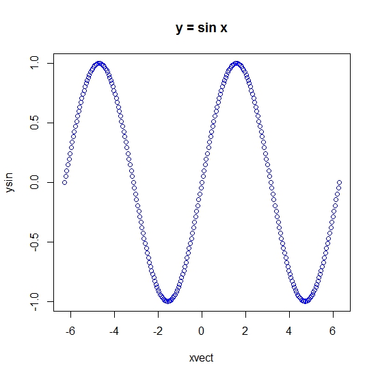
> xvect <-
seq(-2*pi,2*pi,by=pi/64)
> ysin <-
sin(xvect)
> plot.new()
>
plot(xvect,ysin,main="y = sin x",col="blue")
> xtan <-
seq(-pi/4, pi/4, by = pi/64)
> ytan <-
tan(xtan)
>
par(mfrow=c(2,2))
> plot(xvect,
ysin, main = "y = sin x", xlab="x", ylab="y",
col="blue",pch=8)
> plot(xvect,
ycos, main = "y = cos x", xlab="x", ylab="y",
col="red", pch=16)
> plot(xtan,
ytan, main = "y = tan x", xlab="x", ylab="y",
col="forestgreen", pch=20)

Quadratic Fit
>
"Quadratic Fit"
[1]
"Quadratic Fit"
> x <-
c(-3.5,-2.25,-1.15,0,1.15,2.25,3.5)
> y <-
c(10.6,6.3,3.1,2,3.3,6.4,10.4)
>
plot(x,y,main="Quadratic Fit",col="chocolate",pch=20)
> fit <-
lm(y~x+I(x^2))
> cvect <-
coef(fit)
> xrng <-
seq(-3.5,3.5,by=.01)
> yrng <-
cvect[1] + cvect[2]*xrng + cvect[3]*xrng^2
>
lines(xrng,yrng)

Histogram and One Variable Statistics
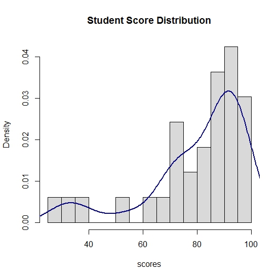
> scores <-
c(99,97,96,95,94,29,39,90,92,92,91,86,84,54,65,72,76,77,81,82,90,33,93,92,89,88,90,98,68,71,73,75,97)
>
"Minimum Score"
[1] "Minimum
Score"
> min(scores)
[1] 29
>
"Maximum Score"
[1] "Maximum
Score"
> max(scores)
[1] 99
>
"Average Score"
[1] "Average
Score"
> mean(scores)
[1] 80.24242
> "Number
of Students"
[1] "Number
of Students"
>
length(scores)
[1] 33
[1] "Basic
Histogram"
> hist(scores)

> "10
Categories and Labels"
[1] "10
Categories and Labels"
> hist(scores,
breaks=10, main="Student Score Breakdown", col="yellow")

> "Fiting
a Distribution"
[1] "Fiting
a Distribution"
> hist(scores,
breaks=10, main="Student Score Distribution",
col="gray85",prob=TRUE)
>
lines(density(scores), lwd=2, col="navy")
Citation:
R Core Team (2015). R: A language and
environment for statistical computing. R Foundation for Statistical Computing,
Vienna, Austria. URL
A personal note,
thank you for your support. My mom and I
are still in recovering/coping mode.
See you next time,
Eddie
This blog is
property of Edward Shore. 2015