HP Prime: Constant Payment Applied to Principal

HP Prime:  Constant Payment Applied to Principal 

Constant Amount Applied to Principal 

In most loans and mortgages,  the amount of payment applying to interest and principal depends on the running balance.  

This program assumes the customer wants an equal portion to apply to principal each payment.   As a result, the payment itself, principal and interest, will vary.  The simple algorithm to amortize this loan is this:

For K=1 to N:

Int =  Bal * I%÷100

Tpmt = Int + CPMT

Bal_k = Bal_(k-1) - CMPT

where:

Bal = balance of a loan

PV = loan amount

CPMT = amount to be applied to principal each payment

I% = interest rate

Int = interest calculated for payment K

Tpmt = total payment for payment K

HP Prime Program CPYMT

The result of CPYMT is a four column matrix with rows:  k, interest in payment k, total payment k, resulting balance.  Keep in mind that program asks for periodic interest rate.  

EXPORT CPYMT()

BEGIN

// 2022-10-24 EWS

// fix 2

HFormat:=1;

HDigits:=2;

// local

LOCAL n,i,p,b,it,tp,k,x;

LOCAL ll,l0,l1,l2,l3,m;

// main

INPUT({n,i,p,b},"Constant Principal",

{"N = ","I%=","PMT=","LOAN="},

{"# of payments",

"periodic interest rate",

"constant payment",

"loan amount"});

l0:={0};

l1:={0};

l2:={b};

FOR k FROM 1 TO n DO

it:=b*i/100;

tp:=p+it;

b:=b-p;

ll:=MAKELIST(x,x,1,n+1,1);

l0:=CONCAT(l0,{it});

l1:=CONCAT(l1,{tp});

l2:=CONCAT(l2,{b});

END;

l3:=CONCAT(ll,l0);

l3:=CONCAT(l3,l1);

l3:=CONCAT(l3,l2);

m:=list2mat(l3,SIZE(l0));

m:=TRN(m);

RETURN m; 

END;

Example

Five year loan of $10,000 where the customer requests an equal amount of principal to be applied each annual payment ($2,000 a year).  The loan rate is 6.99%.

Inputs:

N = 5

I% = 6.99

PMT = 2,000.00

LOAN = 10,000.00

Result:

Year 1:  Interest:  $699.00;  Total Payment:  $2,699.00;  Balance:  $8,000.00

Year 2:  Interest:  $599.20;  Total Payment:  $2,559.20;  Balance:  $6,000.00

Year 3:  Interest:  $419.40;  Total Payment:  $2,419.40;  Balance:  $4,000.00

Year 4:  Interest:  $279.60;  Total Payment:  $2,279.60;  Balance:  $2,000.00

Year 5:  Interest:  $139.80;  Total Payment:  $2,139.80;  Balance:  $0.00

Source

"Constant Payment to Principal Loan"  HP-41 User's Library Solutions: Lend/Lease/Savings  Hewlett Packard.  November 1980

Next week I am going to cover the legendary HP 75C.  

All original content copyright, © 2011-2022.  Edward Shore.   Unauthorized use and/or unauthorized distribution for commercial purposes without express and written permission from the author is strictly prohibited.  This blog entry may be distributed for noncommercial purposes, provided that full credit is given to the author. 

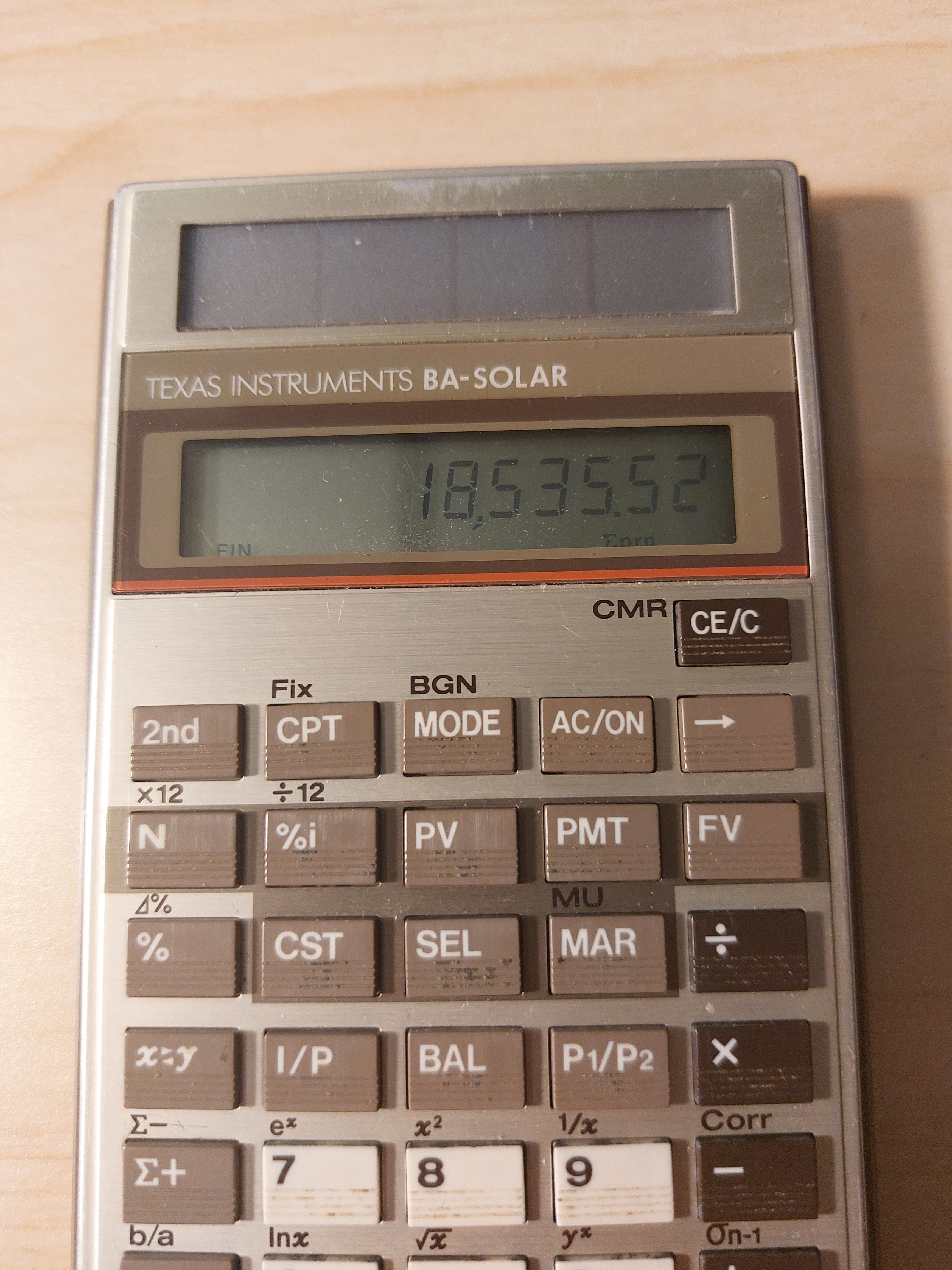
Retro Review: Texas Instruments BA-Solar

Retro Review: Texas Instruments BA-Solar

Finance + Solar + 1980s

Quick Facts

Model:  BA-Solar

Company:  Texas Instruments

Years:  1986 - 1990s; a refresh , BA-35 SOLAR was produced 1996-2000s

Type:  Finance

Batteries: Solar 

Operating Modes:  Chain

Number of Registers: 1, |MEM|

Display:  1 line, 10 digits

Features

The [ MODE ] key is used to toggle between three modes:

FIN Mode:  Time Value of Money  (FIN indicator)

N:  number of payments

%i:  periodic interest rate

PV:  present value

PMT:  payment

FV:  future value

The current cash flow convention is not used, instead the following equation is (I think) used in solving time value of money calculations: 

PV = FV *  SPPV + PMT * USPV

SPPV = single present value factor

USPV = present value annuity factor

We also have amortization functions:

BAL:  balance after any payment

I/P:  interest and principal at any payment

payment_1 P1/P2 payment_2 I/P:  cumulative interest and principal

There are ×12 and ÷12 aids, but we still have to press [ N ] and [ %i ] to register the values, they are not automatic.  

STAT Mode:  Statistics  (STAT indicator)

The BA-SOLAR (and the later BA-35 SOLAR) has both single variable statistics and linear regression.

In linear regression, use the [x<>y] key to change between x and y.   The key will also be used to switch between results.  

Prediction values can be calculated with x' and y'.

The equation used for linear regression is y = a*x + b,  a = slope, b = intercept.

Profit Mode (no indicator)

The profit mode makes the following solver available:

CST:  cost

SEL:  sell

MAR:  margin

MU:  markup

Functions Available in All Modes

Percent Calculations (%):

Add %:  x [ + ] y [ % ] [ = ]

Subtract %:  x [ - ] y [ % ] [ = ]

Multiply %:  x [ × ] y [ % ] [ = ]

Percent Ratio:  part [ ÷ ] whole [ % ] [ = ]

Percent Change:  new [ 2nd ] ( ⊿% ) old [ = ]

rate >EFF payments/year:  convert to effective rate

rate >APR payments/year:  convert to APR/nominal rate

Mathematics:

Natural logarithm and antilogarithm:  ln x, ^x

Square and square root

Power

Reciprocal

Final Thoughts

This is a great basic financial calculator.  I have both the BA-SOLAR and BA-35 SOLAR.   To be honest, I like the keyboard of the original BA-SOLAR better, the keys feel a bit more solid and responsive.  Even though they are no longer in production, the BA-SOLAR is still reasonably available on sites such as eBay and other online stores.  

Source:

Woerner, Joerg.  "Texas Instruments BA-SOLAR"  Last Updated December 5, 2001.   http://www.datamath.org/Sci/Modern/BA-SOLAR.htm   Retrieved May 19, 2022.

Eddie

All original content copyright, © 2011-2022.  Edward Shore.   Unauthorized use and/or unauthorized distribution for commercial purposes without express and written permission from the author is strictly prohibited.  This blog entry may be distributed for noncommercial purposes, provided that full credit is given to the author. 

Retro Review: Texas Instruments BA II Financial Calculator (1984)

Retro Review:  Texas Instruments BA II Financial Calculator (1984)

BA II:  Finance Mode

BA II:  Statistics Mode

Company:  Texas Instruments

Mode:  BA II

Year: 1984

Batteries:  2 A76 batteries, or 2 357 batteries

Memory Registers: 1  (only 1, other variables can’t be recalled)

Where’s the Plus?

This review isn’t about the BA II Plus, this is an earlier model.  I purchased the BA II from a box in the Azusa Swap Meet last Sunday (January 28, 2017) for 1 dollar.  Thankfully the previous owner did not leave the old batteries so I didn’t have to worry about battery corrosion.  The previous owner (or one of them) has their name and address on the calculator.  Obviously for privacy issues I took of a couple of stickers containing the address.

The BA II is the second generation of the TI Business Analyst II (released in 1978).  The first generation of the Business Analysist II sold for $40-$45 new.  The Datamath page for the TI Business Analyst II:  http://www.datamath.org/Sci/Slimline/Business-Analyst-II.htm

Three Modes

The BA II has three modes which cycle by the key sequence [ 2^nd ] [ FIX ] (Mode):

‘Profit Mode (no indicator):  Profit Margin mode.  Only the [CST] (cost), [SEL] (selling price), and [MAR] (margin) keys are active.  Solve for the following variables by preceding the key by [ 2^nd ].

‘Finance Mode (FIN indicator):  Time Value of Money mode.  Only the [ N ], [ %i ], [ PMT ], [ PV ], and [ FV ] keys are active.  Solve for the following variables by preceding the key by [ 2^nd ] or if you are working with beginning of period annuity by using [DUE] instead.  Also, the P/I (Principle and Interest of a single payment) and Acc/Bal (accumulated interest and balance) are also available.

‘Statistics Mode (STAT indicator): Statistics Mode, including linear regression.  The equation is y = a + b*x where a is the intercept and b is the slope.  Mean, deviation, and predictions are also available.

Other Functions

Percent Change:  Δ% has the syntax (new number [ 2^nd ] [ % ] (Δ%) old number [ = ])

Fix Modes:  FIX 0-7 will fix the number to that decimal places.  Using FIX 8-9 engage floating mode.

Early Installment Weirdness

1. There is no [CPT] button like it would be prevalent on later Texas Instruments financial calculators. 

2. The sign of cash flow conventions are not followed.  See the example below:

Example:  Calculate the monthly payment of a $174,000 loan.  The loan is for 30 years, 4.65% annual interest, and no balloon payment (FV = 0).  Assume that FIX 2 is in affect and Finance mode is selected.

Remember N is the number of payments and %i is the periodic interest rate (in this case monthly).

Keystrokes:

174000 [PV]

30 [ * ] 12 [ = ] [ N ]

4.65 [ ÷ ] 12 [ = ] [ %i ]

[ 2^nd ] [ PMT ]

The result of 897.21.  (There is no negative sign for outflow like in more current financial calculators, including the HP 12C)

Principal/Interest at the 60^th payment:

Keystrokes:

60 [ 2^nd ] [ x<>y ] (P/I)

Returns:  280.11 (principal) [ x<>y ] 617.10 (interest)

Accumulated Interest and Balance after 60 payments:

Keystrokes:

60 [ 2^nd ] [ K ] (Acc/Bal)

Returns: 38804.61 (accumulated interest) [ x<>y ] 158,972.13 (balance)

My recommendation is to write down your answers and key in the time.

Final Verdict

The BA II is a good entry-level financial calculator.  Being it is a 1984, the patience will be required for some calculations. 

Eddie

This is Edward Shore, 2017

Sharp EL-738: A Short Tutorial

Sharp EL-738:  A Short Tutorial

This is a short tutorial on how to use some of the common features of the Sharp EL-738 financial calculator.  There was a request for a video tutorial in the comments, however given the time frame I am able to work with, I think I can write a tutorial and cover more faster.  So hope this helps!

The full manual is here:  http://sharpcalculators.com/images/Manuals/Financial/EL738F_Manual_Branded.pdf

To see my review back in August last year, click here:

http://edspi31415.blogspot.com/2015/08/review-sharp-el-738f-financial.html

Let’s get to it.

Set Decimal Settings

To Fix 2 Mode:  [SET UP], 0 (DSP), 0 (TAB), 2

To Float (B) Mode:  [SET UP], 0 (DSP), 3 (FLO_A)

The difference between FLO_A (option 2) and FLO_B is the limit of how small a number can be before the calculator switches to scientific notation.  .000000001 for A and .01 for B.

Time Value of Money

To set the number of payments:  press [2ndF] [I/Y] (P/Y).  Enter the payments per year and press [ENT].  You can enter compounding periods (C/Y) per year separately. 

Toggle Begin/End Mode:  [2ndF] [ FV ] (BGN/END).  Beginning mode is indicated by “BGN” in the display.

Clear the Financial registers:  [2ndF] [MODE] (CA).  Caution: This sets the P/Y to its default value of 1. 

Calculation:  Enter each of the date and press the appropriate financial variable (N, I/Y, PV, PMT, or FV).  To calculate, press [COMP] then the financial variable. 

Example:  Find the monthly payment of a $160,000 loan to be paid back in 15 years with 3.5% interest. 

If not already, set P/Y to 12 and calculator to END mode (see the above).

160000 [ PV ]

15 [2ndF] [ N ] (xP/Y) [ N ] 

3.5 [I/Y]

0 [ FV ]

[COMP] [PMT]

Result:  -1143.81

Amortization

Press [AMRT].   Enter the first period (P1) then press [ENT].  Scroll down [ ↓ ] and enter the second period (P2) then press [ENT].  Scroll down for the following results (calculated automatically):  BALANCE, ΣPRINCIPAL (amount of principal paid in period range specified), ΣINTEREST (amount of interest paid in period range specified).

Take the last example and set P1 to 1 and P2 to 24.  After two years:

[AMRT] 1 [ENT] [ ↓ ]

24 [ENT] [ ↓ ]

Result:  BALANCE:  143,191.61   [ ↓ ]

Result:  ΣPRINCIPAL = -16808.39  [ ↓ ]

Result:  ΣINTEREST = -10643.05

Days Between Dates

Press [DATE].   M-D-Y 1 represents the beginning date.  M-D-Y 2 represents the ending date.  DAYS is the number of days between the two dates.  This assumes the U.S. date system is set up.

Scroll up and down.  Enter two of the three variables and press [COMP] to solve for the third.

Example:  A bond is issued on 7/1/2016. The bond is to be repaid in 120 days.  When is the bond supposed to be repaid?  Assume an actual calendar.  ([2ndF] [COMP] (360/ACT) toggles calendar counting mode)

[DATE]

For M-D-Y 1:  07, 01, 2016 [ENT]

[ ↓ ], [ ↓ ]

For DAYS:  120 [ENT]

[ ↑ ] to M-D-Y 2, press [COMP]

Result:  10/29/2016

Cash Flows

To clear all cash flows:  Press [2ndF] [ENT] (CLR-D).  I also recommend setting P/Y to 1 (pressing [2ndF] [MODE] (CA) will do it)

To enter cash flows:  Enter the cash flow, press [ ENT ].  (Don’t be in any menu or worksheet)

To enter cash flows with frequency greater than 1:  Enter the cash flow, press [(x,y)], enter the frequency, press [ ENT ].

To calculate NPV (net present value):  press [2ndF] [CFi] (CASH).  Enter the periodic rate at the RATE(I/Y)=, press [ENT], then [ ↓ ], and press [COMP] at the NET_PV prompt.

To calculate IRR (initial rate of return):  press [2ndF] [CFi] (CASH).  Press [COMP] at the RATE(I/Y)= prompt.   For this purpose, ignore the NET_PV register.

Example:   Calculate the NPV and IRR of the following cash flows:

Flow #	Amount
CF0	-$10,000
CF1	$5,000
CF2	$2,000
CF3	$5,000

For NPV, assume a return rate of 10%.

Cash Flows:

[2ndF] [MODE] (CA)

[2ndF] [ENT] (CLR-D)

10000 [+/-] [ENT]   (Display:  DATA SET: CF 0.00)

5000 [ENT] (Display:  DATA SET: CF 1.00 (and so on))

2000 [ENT]

5000 [ENT]

Net Present Value:

[2ndF] [CFi] (CASH)

RATE I/Y=:  10 [ENT]

[ ↓ ]

NET_PV=:  [COMP]

Result:  -45.08

Internal Rate of Return:

[ ↑ ]

RATE(I/Y)=:   [COMP]

Result:  9.74

Some quick instructions about depreciation and statistics:

Depreciation

The EL-738 has three depreciation modes:  Straight Line (SL), Sum of the Years Digits (SYD), and Declining Balance (DB).  To change the depreciation mode, press [SETUP], 2 and then:

0 for SL, 1 for SYD, 2 for DB.

To the Depreciation worksheet:  Press [DEPR].

Mode:  If the Declining Balance Deprecation Mode is set, enter the rate (for 200%, enter 200, press [ENT])  [ ↓ ]

Life (N):  Enter the number of years of the life of the asset, [ENT], [ ↓ ]

Start Month:  Enter the month when the asset is acquired (1 = January, 2 = February, etc), [ENT], [ ↓ ]

COST (PV): Cost of the asset, [ENT], [ ↓ ]

SALVAGE (FV):  Salvage value of the asset, [ENT], [ ↓ ]

YEAR=  Enter year of depreciation that you want to analyze, [ENT], [ ↓ ].

The next three lines are calculated: DEPRECIATE (the deprecation for the year, RBV (remaining book value), RDV (remaining depreciation value)

Statistics

To enter statistics mode, press [MODE], 2.  Select statistics type:

0:  SD, single variable

1:  LINE: linear regression, y = a + bx

2:  QUAD: quadratic regression, y = a + bx + cx^2

3:  EXP:  exponential regression, y = a * e^(bx)

4:  LOG:  logarithmic regression, y = a + b * ln x

5:  PWR:  power regression, y = a * x^b

6:  INV:  inverse regression, y = a + b/x

Clearing Data:  [2ndF] [DATA] (CLR D)

Entering Data:  x [(x,y)] y/freq [ENT] (DATA)

Recall variables:  [ALPHA] [(appropriate key)] [ = ]

Examples:

Mean:  μx: [ALPHA], 4;  μy: [ALPHA], 7

Sample Deviation:  sx: [ALPHA], 5; sy:  [ALPHA], 8

Regression variables a, b, c, r:  [ALPHA] [ ÷ ], [ DEL],. [ × ], [ ( ], respectively

  

You can find detailed instructions for the other operations (cost/sell/margin worksheet, Δ% worksheet, bond worksheet, depreciation, scientific functions), plus more examples, in the manual:  http://sharpcalculators.com/images/Manuals/Financial/EL738F_Manual_Branded.pdf

This blog is property of Edward Shore, 2016.