Retro Review: Casio BF-80

Retro Review:   Casio BF-80

A folding calculator with easy-to-calculate finance prompts.  

Quick Facts

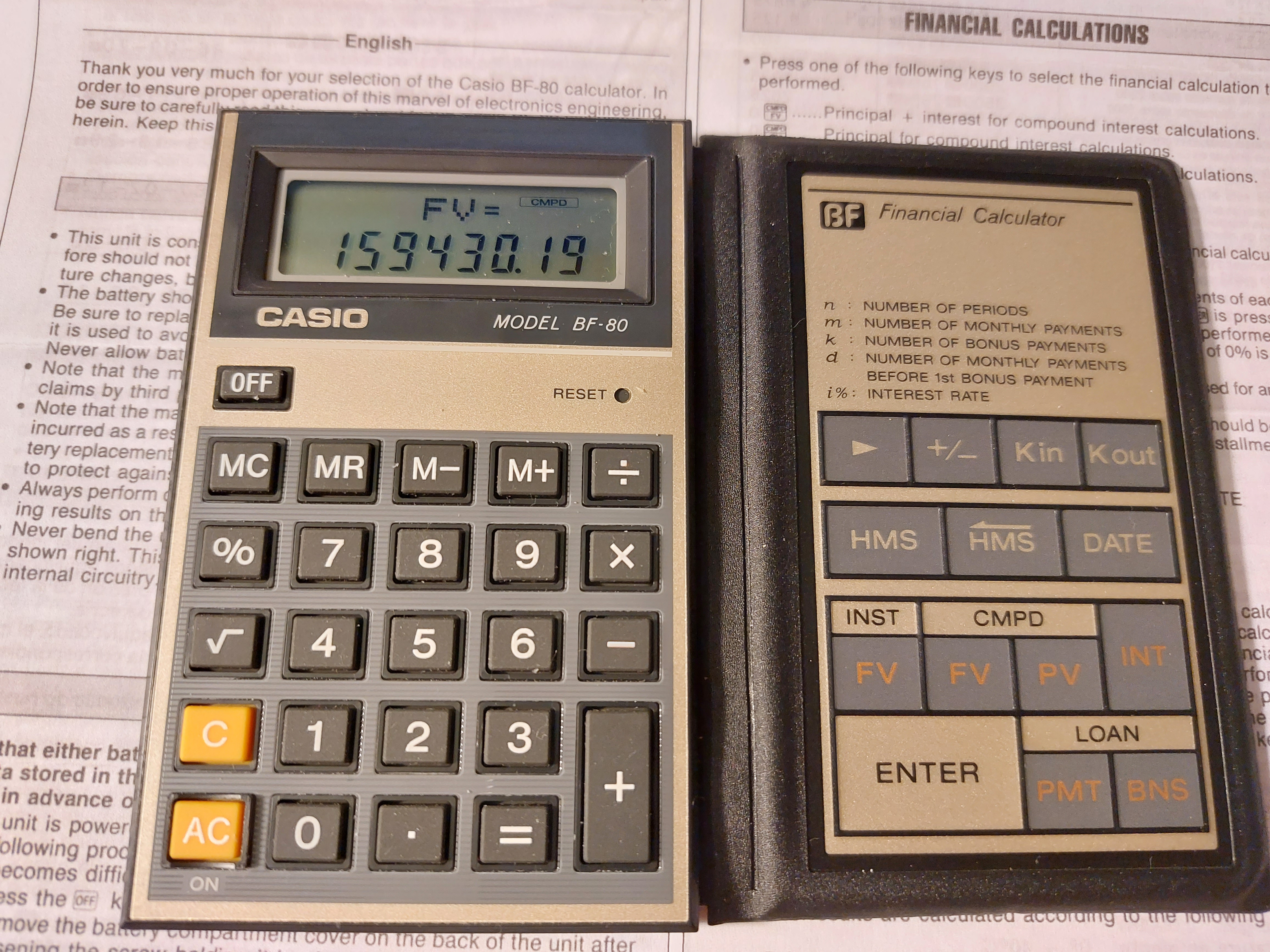
Model:  BF-80  (Easy Banker Financial)

Company:  Casio

Years:  1985 (production run is probably the late 1980s)

Type:  Finance

Batteries: 1 x CR-2016

Operating Modes:  Chain

Number of Registers: 2 User registers:  M,  Kin/Kout 

Display:  2 lines

Features

The BF-80 is a dual-leaf calculator.  On the left side, you have a regular four-function calculator, including memory functions, percent, and the square root function.

On the right side is where all the financial functions the BF-80 are located:

[ Kin ]/[ Kout ]:  The BF-80's other user memory register.  Unlike register M, there is no register arithmetic.

[ HMS ]/[ <HMS ]:  Convert decimal to/from hours-minutes-seconds.  Use the [ HMS ] key to enter parts of time.  

Example:  Add 3.5 hours to 11:30:00

11 [ HMS ] 30 [ HMS ] [ + ] 3.5 [ = ] 

Result:  15°0°0 (15:00:00)

[ DATE ]:  The date key leads two of my favorite functions of all time:  days between dates and calculating a future date.   The format is yy - mm - dd  (no dashes for 21st century dates).  Years are entered as four digits, from 1901 to 2099.  

For most, if not all, calculators, the cash flow convention is not used.  

INST-FV:  Calculates the future value of an annuity.  Interest rate is entered as periodical rate. Note that deposits are made at the beginning of each period (annuity due).  The INST indicator turns on. 

Example:  I pay $500 a month in an account that pays 5% interest for 10 years.

[ INST FV ]   (INST indicator is on)

PMT?  500 [ ENTER ]

i%?  5 [ ÷ ] 12 [ = ] [ ENTER ] 

n?  10 [ ÷ ]  12 [ = ] [ ENTER ]

FV= 77964.641

Pressing [ INT ] gives the interest earned:  17964.641.

CMPD-FV:  Calculates the future value of a lump sum (present value).  The CMPD indicator turns on, and INT gives the accumulated interest.

CMPD-PV:  Calculates the present value of a future lump sum (future value).  The CMPD indicator turns on, and INT gives the accumulated interest.  

Both CMPD calculations use this equation:

FV = PV * (1 + i%)^n

LOAN-PMT:  Calculates the monthly payment of a loan due at the end of each month.  The loan is to paid without a balloon payment.  The LOAN indicator turns on.

PV?:  amount to be financed

i%?:  annual interest rate

m?:  number of monthly payments

Example:  What is the monthly payment of $8,293.00 loan with 6% interest over 6 years?

[ LOAN PMT ] (LOAN indicator is on)

PV? 8293 [ ENTER ]

i%?  6 [ ENTER ] (no dividing by 12 in LOAN mode)

m? 6 [ × ] 12 [ = ] [ ENTER ] (still enter the number of months)

PMT = 137.43896

Pressing [ INT ] gives the accumulated interest paid on the loan:  -1602.6051

LOAN-BNS:  Calculates the bonus payment of a separate (side) loan given the number of bonus payments and it's cycle.

k = number of bonus payments

d = number of months to the first bonus payment

PV = bonus loan amount

i% = annual interest rate of the bonus loan

Example:  What is the payment of a bonus loan of $4,412.00 with 3% interest.  The firs bonus cycle is every 3 months from the loan date, with 15 bonus payments.

[ LOAN BNS ]  (LOAN indicator is on)

PV?  4412 [ ENTER ]

i%?  3 [ ENTER ]  (annual rate, like LOAN-PMT)

k?  15 [ ENTER ] (number of bonus payments)

d?  3 [ ENTER ] (number of months prior to the first bonus payment)

BNS = 328.21123

Pressing [ INT ] gives the accumulated interest:  -511.16857

I guess that this is for loans where payments are due every few months instead of every month.  

The Percent Key

The percent key on the BF-80 works like most Casio calculators with a percent key.   

To add a percent:  n [ × ] p [ % ] [ + ]

To subtract a percent:  n [ × ] p [ % ] [ - ]

To find a percent ratio:  part [ ÷ ] whole [ % ]

Percent change:  new [ - ] old [ % ]

A Neat Calculator - An 1980s Version of a Smartphone App 

For it's time, the BF-80 offers calculator with quick, prompting calculations for the on-the-go business and finance student or profession.  Today, in the 2020s, the calculator of this time definitely would  be a smartphone app.  

Surprisingly buying a BF-80 was incredibly reasonable.   

Coming up:

July 11 - July 15, 2022:  TI-58 and TI-59 Week

Next Regular Blog:  July 10, 2022, then  July 23, 2022

Eddie

All original content copyright, © 2011-2022.  Edward Shore.   Unauthorized use and/or unauthorized distribution for commercial purposes without express and written permission from the author is strictly prohibited.  This blog entry may be distributed for noncommercial purposes, provided that full credit is given to the author. 

Retro Review: Casio FC-1000 Financial Consultant

Retro Review:   Casio FC-1000 Financial Consultant

Birthday post!

Quick Facts:

Model:  FC-1000 Financial Consultant

Company:  Casio

Years:  1988-early 1990s

Type:  Finance and Graphic

Batteries:  3 x CR-2025

Memory: 2,470 programming steps

Contrast wheel 

Like the Casio fx-7500G, the FC-1000 is a foldable calculator which is very small and light.  

Features

The main modes of the FC-1000 are come in two categories:  system modes and calculation modes.

System Modes

Run Mode (Mode 1):  This mode is for calculations and running programs.

Write Mode (Mode 2):  This mode is for writing programs, in one of 10 slots, Prog 0 to Prog 9.

Program Clear Mode (Mode 3):  Erase programs in this mode.  Clear all programs by pressing [ SHIFT ] [ DEL ] ( Mcl ).

Calculation Modes

Financial Mode (Mode 4):  This mode is for financial calculations including time value of money (simple/compound/monthly C.I.), amortization, D.C.F. (discounted cash flows including NPV, IRR, NFV), bonds, depreciation, and cost/sell/margin.  The financial calculations are accessed by pressing the [ MENU ] key.   One of the great things of the FC-1000 is that it has a big screen to list variables and menu choices.  

Linear Regression Mode (Mode 5):  This mode fits bivariate data to the equation y = a + bx.  

SD Mode (Mode 6):  Single variable statistics

Mathematical Functions

The FC-1000 has a set of mathematical functions tailored to financial calculations:

*  powers and roots

*  logarithms

*  integer and fraction parts

*  factorials of positive integers

*  days between dates

How to figure out how to calculate days between dates:  

month_before [ DATE ] day_before [ DATE ] year_before [ DATE ] [ - ]

month_after [ DATE ] day_after [ DATE ] year_after [ DATE ]

If a two digit year is entered, it is implied that the year is 19##.  Thankfully four digits years are allowed, so this calculator can be used in the 21st century.   (Trivia:  I will be alive 16,436 days today using the 365 day mode).

The date separate is indicated by a forward slash.  

Programming 

The FC-1000 uses the Casio basic programming language.  The following commands available are:

Comparisons and the jump command:

[ test ] ⇒ [ do if true ] : or ◢  [ skip to here if false ]

Goto and label commands (Lbl 0-9)

Count jumps Isz (increment and skip on zero) and Dsz (decrement and skip on zero)

We can also store values in financial variables that are accessed through the menu system.  

As mentioned before, the space has a capacity of 2,470 steps over 10 program slots. 

Graphing

The FC-1000 has graphing, but is limited to certain financial applications:  bonds, amortization, and depreciation.   Depending on what type of graph, pressing [ Trace ] will highlight the next period, and [ Shift ] [ Trace ] will rotate between different points of data.

For instance, in bonds, the [ Shift ] [ Trace ] combination rotates between price (PRC), coupon (CPN), and redemption value (RDV).

In amortization, the cycle is interest (INT), principal (PRN), and the nth payment (n).

In depreciation, the cycle is the year's depreciation (Depr) and year (n).  

Closing Thoughts

I love the form factor of the FC-1000 and how compact the calculator is.   However, the calculator is light weight and extra care is a must.  I wish the graphing module allowed us to graph functions and added statistical graphs.   

The FC-1000 can be difficult to collect, hence prices may be higher than a lot of vintage calculators.  

Until next time,

Eddie

All original content copyright, © 2011-2022.  Edward Shore.   Unauthorized use and/or unauthorized distribution for commercial purposes without express and written permission from the author is strictly prohibited.  This blog entry may be distributed for noncommercial purposes, provided that full credit is given to the author. 

Review and Instruction: Senario FC-500 Financial Calculator

Review and Instruction: Senario FC-500 Financial Calculator

Announcement:  Twelve Days of Integrals

In spirit of the Twelve Days of Christmas, I present the Twelve Days of Integrals:  starting December 25, 2021 to January 5, 2022.  I hope everyone has a happy, health, and sane holiday season!

Now on to the review.

Review: Senario FC-500 Financial Calculator

Quick Facts

Model: FC-500

Company: Senario

Years: ??, sometime in the 2010s?

Memory Register:  1 user memory with separate registers

Battery:  Battery, 2 x LR44

Screen:  12 digits

Logic:  Chain

I purchased the Senario FC-500 on eBay for relatively cheap.  The one I purchased did not come with an instruction manual, and I couldn't find one online.   

Through playing with the calculator and research with other financial calculators, the FC-500 models itself after the Hewlett Packard HP 12C.  

What makes this financial calculator a little unique is the wonderful presence of 40 U.S.-metric conversions.   The FC-500 is a feature rich financial calculator.  

I have yet to find instruction on how to change the number of decimal points displayed, if that is even available.  Most financial calculators default to the 2 decimal point setting, and that would be the expected setting.  This would be one of my sticky points for the FC-500, the other would be lack of user memory registers.  

The cash flow convention is followed:  positive for cash inflows (deposits and receipts), negative for cash outflows (payments).  The key with a magnifying glass over a document, which is located on the second row, sixth key (right-most key) is the compute/calculate key.  On this blog I will designate this key as the [(search)] button.

Features

*  Time Value of Money

*  Depreciation (Straight Line, Sum of the Years Digit, Declining Balance)

*  Sell/Cost/Margin (SEL, CST, MGN)

*  Interest Conversion:   Effective vs Nominal (APR)

*  Percent Calculations (%, percent change, % of total)

*  Currency conversions

*  Tax calculation (TAX+ and TAX-) 

*  Days between dates and date calculations (four digit years)

*  Statistics including Linear Regression

The rest will be an instruction sheet for those who are looking for a manual.  For anything I missed, you may want to look at the HP 10BII+ or HP 12C manual and it may fill the rest of the gaps.   Hope this helps.

Operating the FC-500

Time Value of Money (TVM)

PV:  present value

n:  number of payments, ×12

i:  periodic interest rate, ÷12

PMT:  payment

FV:  future value

Magnifying glass, designated as [(search)]:   Solve/CPT

B/E:  Beginning/End Toggle

Cash flow convention is followed

Example:

PV:  0.00

n:  3 years 

i:  3.86% compounded monthly

payment:  $50.00 per month

0 [ PV ]

3 [SHIFT] (×12)

3.86 [SHIFT] (÷12)

50 [+/-] [ PMT ]

[(glass)] [ FV ] returns 1,905.11893693

Amortization Procedure

1.  Enter n, i, PV, and any balloon amount in FV.

2.  Compute PMT.

3.  Enter period 1 to n, second period, press [SHIFT] (AMORT)

4.  Accumulated Interest,  [ X←→Y ], Accumulated Principal

5.  [ RCL ] [ PV ]: remaining balance

6.  [ RCL ] [ n ]: number of payments amortized

7.  To do the next batch, press [ SHIFT ] (AMORT), repeat steps 4 through 6

Example:

Loan:  $189,000.00

I/YR:  4.8% compounded monthly

Years: 20 years of monthly payments

No balloon payment

Amortize the first 2 years of 12 month payments

189000 [ PV ]

20 [SHIFT] [ ×12 ]

4.8 [SHIFT] [ ÷12 ]

0 [ FV ]

[(search)] [ PMT ] returns -1,226.529641804

First 12 Payments

0 [ n ] 12 [SHIFT] (AMORT)

Accumulated Interest:  -8,946.10891465

Accumulated Principal: [ X←→Y ], -5,772.24650183

Balance:  [ RCL ] [ PV ],  183,227.753498

Second 12 Payments

12 [SHIFT] (AMORT)

Accumulated Interest:  -8,662.86358088

Accumulated Principal: [ X←→Y ], -6,055.4918356

Balance:  [ RCL ] [ PV ],  177,172.261662

EFF/NOM conversion

Convert from NOM (APR) to EFF

payments per year [ n ]

nominal rate [ NOM ] 

[(search)] [ EFF ] 

Example:  NOM = 6%, payments per year = 24

24 [ n ]  6 [ NOM ]  [(search)] [ EFF ] returns 6.17570442629

Convert from EFF to NOM (APR)

payments per year [ n ]

nominal rate [ EFF ] 

[(search)] [ NOM ] 

Example:  NOM = 6%, payments per year = 24

24 [ n ]  6 [ EFF ]  [(search)] [ NOM ] returns 5.83397001049

Percent Change

old [ X←→Y ] new [ Δ% ]

Example:   4750 [ X←→Y ] 4200 [ Δ% ] returns -11.5789473684

Days Between Dates

first date [ X←→Y ] second date [SHIFT] (ΔDAYS)

Example:  3.141977 [ X←→Y ] 12.092021 [SHIFT] (ΔDAYS) returns 16,341

(M.DY year mode)

(March 14, 1977  to December 9, 2021)

Percent Total

whole [ X←→Y ] part [ %T ]

Example:  85 [ X←→Y ] 41 [ %T ] returns 48.2352941176

Date Addition

date [ X←→Y ] number of days [SHIFT] (DATE)

Day number:  1:  Monday to 7: Sunday

Example:  Determine the date 90 days from November 15, 2021?  (M.DY year mode)

11.152021 [ X←→Y ] 90 [SHIFT] (DATE) returns 2.132022-7

(Sunday February 13, 2022)

Tax Addition and Subtraction (Sales Tax)

To set the tax rate:  rate [SHIFT] (RATE SET)

To add the tax rate:  [TAX+]:   x∙(1+rate/100)

To subtract the tax rate:  [TAX-]:  x/(1+rate/100)

Example:  Set rate at 9.5%

200 [TAX+] returns 219

150 [TAX-] returns 136.986301369

Unit Conversions 

40 conversions

Use the blue keys:

[ ← ]:  metric to US

[ → ]: US to metric

Statistics - Linear Regression

Date:  x [ X←→Y ] y [ Σ+ ]

Registers used:   (not used for other purposes)

[ RCL ] [ 1 ]: N

[ RCL ] [ 2 ]: Σx

[ RCL ] [ 3 ]: Σx^2

[ RCL ] [ 4 ]: Σy

[ RCL ] [ 5 ]: Σy^2

[ RCL ] [ 6 ]: Σxy

Depreciation

[ n ]:  life of the asset in years

[ PV ]:  cost

[ FV ]:  salvage value, if any

[ i ]:  rate (for declining balance only)

year # [ SHIFT ] ( SL ):  Straight Line Depreciation  (press [ X ←→ Y] for book value)

year # [ SHIFT ] ( SOYD ):  Sum of the Year's Digits Depreciation  (press [ X ←→ Y] for book value)

year # [ SHIFT ] ( SL ):  Declining Balance Depreciation  (press [ X ←→ Y] for book value)

Simple Interest

n:  number of days

i:  annual interest rate

PV:  principal amount

Enter 0 in PMT and FV

Press [SHIFT] (INT) for simple interest

Example:

Calculate the simple interest of a 30-day loan of $1,400.00.  The annual rate is 6.5%.

1400 [ PV ]

30 [ n ]

6.5 [ i ] 

0 [ PMT ], 0 [ FV ]

[SHIFT] (INT) returns -7.583333333333  (360-day year)

[ X ←→ Y] -7.7945205479 (365-day year)

Eddie

All original content copyright, © 2011-2021.  Edward Shore.   Unauthorized use and/or unauthorized distribution for commercial purposes without express and written permission from the author is strictly prohibited.  This blog entry may be distributed for noncommercial purposes, provided that full credit is given to the author. 

Fun with the Sharp EL-5500 III

Fun with the Sharp EL-5500 III

See my review for the EL-5500 III here:  http://edspi31415.blogspot.com/2017/01/retro-review-sharp-scientific-computer.html

Even though the EL-5500 III has one programming space, we can fit many programs in it.  One of the great features is that how programs take relatively little space.  Obviously you can change the line numbers, the sequence of lines are most important.

Euclid Algorithm – RUN 10

10 PAUSE “GCD: A>B”

18 INPUT “A: “; A, “B: “; B

20 C = A – INT(A/B)*B

30 IF C = 0 THEN 40

32 A = B

34 B = C

36 GOTO 20

40 PRINT “GCD = “; B

46 END

My first program on the EL-5500 III.  We can probably make the coding more efficient.  PRINT with a proceeding WAIT pauses execution until [ ENTER ] is pressed.

The command END ends the program execution and allows the space to have more than one routines.

Examples:

A: 100, B: 20.  Result:  GCD = 20

A: 63, B: 60.  Result:  GCD = 3

Binomial Expansion – RUN 50

50 PAUSE “(Ax + B)^n”

55 INPUT “A: “;A, “B: “;B, “N: “,N

60 FOR I=0 TO N

65 C = FACT(N) / (FACT(I) * FACT(N-I))

70 T = C * A^(N-I) * B^I

75 PRINT T; “*x^”; N-I

80 NEXT I

85 END

The command PAUSE shows the text for about 0.85 seconds.

This program displays each coefficient one at time.

Example:  A = 3, B = -2, N = 3.  Expand (3 – 2x)^3.

Result:  27, -54, 36, -8  (27x^3 – 54x^2 + 36x – 8)

Days Between Dates – RUN 100

100 PAUSE “Days between Dates”

112 INPUT “M1:”; M1, “D1:”; D1, “Y1:”; Y1

113 INPUT “M2:”; M2, “D2:”; D2, “Y2:”; Y2

115 M = M1: D = D1: Y = Y1

117 GOSUB 140

119 F1 = F

121 M = M2: D = D2: Y = Y2

123 GOSUB 140

125 F2 = F

127 N = F2 – F1

129 PRINT “# DAYS: “; N

131 END

140 IF M > 2 THEN 150

142 X = 0: Z = Y – 1

144 GOTO 160

150 X = INT(.4 * M + 2.3): Z = Y

160 F = 365 * Y + 31* (M – 1) + D + INT(Z/4) – X

165 RETURN

If I had it my way, every calculator that isn’t a basic 4-function calculator will have a Days Between Dates function.

Example:  November 4, 1986 to January 12, 2017

M1:  11, D1: 4, Y1: 1986 

M2: 1, D2: 12, Y2: 2017

Result:  11,027

Power of a Complex Number – RUN 200

This calculates (a + bi)^n

200 PAUSE “(A + Bi)^n”

203 INPUT “A: “;A, “B: “;B, “n: “;N

205 IF A<>0 THEN 210

207 A = A^N: GOTO 220

210 R = √(A^2 + B^2)^N

212 T = ATN(B/A)*N

214 A = R * COS T

216 B = R * SIN T

220 PRINT A; “+”; B; “i”

225 END

The command <> means not equals (≠) and ATN is the arctangent function.

Examples:

(2 + 3i)^3:  A = 2, Bi = 3.  Result: -46 + 9i

(-5 + i)^2:  A = -5, Bi = 1.  Result: 24 – 10i

Error Function Approximation – RUN 250

250 PAUSE “APPROX ERF(X)”

252 CLEAR

254 DIM A(3)

256 E = 0

260 INPUT “X > 0 : “; X

262 T = RCP(1 + .47047 * X)

270 FOR I = 1 TO 3

272 READ A(I)

274 E = E + A(I) * T^I

276 NEXT I

280 DATA .3480242, -.0958798, .7478556

290 E = 1 – E * EXP(-(X^2))

292 PRINT “ERF : “, F

294 CLEAR

296 END

Use the command CLEAR to clear all the variables.  At this point, I will use this command both at the beginning and end of calculations.  The command RCP is the reciprocal.  Finally, EXP is from e^x function, not the [EXP] key.

Example:

x = 0.53, erf ≈ 0.546455764

x = 0.88, erf ≈ 7.86708E-01 = 0.786708

Keep in mind this approximation is accurate 2.5 parts in 10^-5.

Source:  Smith, Jon M.  Scientific Analysis on the Pocket Calculator  John Wiley & Sons: New York. 1975.  ISBN 0-471-79997-1

Simpson’s Rule – RUN 300

Calculates the numeric integral ∫ f(x) dx from x = L to x = U.

You can edit the function at line 342.  In BASIC-PRO mode, call up line 342 by LIST 342.  Edit as desired.

300 PAUSE “Simpsons Rule”

302 CLEAR

304 INPUT “LOWER: “; L, “UPPER: “; U, “PARTS (even): “; N

306 RADIAN

308 X = L: GOSUB 340: T = F

310 X = U: GOSUB 340: T = T + F

314 H = (U – L)/N

320 FOR I = 1 TO N-1

322 X = L + I * H: GOSUB 340

324 R = I/2 – INT(I/2)

326 IF R = 0 THEN LET T = T + 2*F

328 IF R <> 0 THEN LET T = T + 4*F

330 NEXT I

332 T = T * H/3

334 PRINT “Integral: “, T

336 CLEAR

338 END

340 REM f(x)

342 F = [insert f(X) here]

344 RETURN

Note:  I finally learn why LET is included in BASIC.  In an IF-THEN statement, if you want to assign a value or calculation to a variable, you will need a LET command.

I use a REM (remark) command on line 340.  REM is for comments and nothing said after REM is executed.

Examples:

342 F = X^2 – 1

L = -2, U = 2, N = 14.  Result:  1.333333334 (Actual: 4/3 ≈ 1.333333333)

342 F = √(X – 1)

L = 2, U = 3, N = 14.  Result: 1.218951372 (Actual:  ≈ 1.2158951416)

Dancing Star Demo – RUN 400

400 PAUSE “Dancing Star Demo”

405 CLEAR

410 S$ = “         “  (9 spaces)

415 FOR I = 1 TO 48

420 N = RND 7 + 1

425 T$ = MID$(S$, 1, N-1) + “*” + MID$(S$, N+1, 9-(N+1))

430 WAIT 15: PRINT T$

440 NEXT I

445 BEEP 3: CLEAR: END

This is just show a dancing asterisk (*) on the screen.

WAIT 15: PRINT T$:   This causes the string T$ after a quarter of a second.  WAIT operates in 1/60 seconds.

RND n:  This is the random command.  If n = 1, the result is between 0 and 1. 

BEEP n:  This makes the EL-5500 III beep n times. 

Eddie

This blog is property of Edward Shore, 2017.

Sharp EL-738: A Short Tutorial

Sharp EL-738:  A Short Tutorial

This is a short tutorial on how to use some of the common features of the Sharp EL-738 financial calculator.  There was a request for a video tutorial in the comments, however given the time frame I am able to work with, I think I can write a tutorial and cover more faster.  So hope this helps!

The full manual is here:  http://sharpcalculators.com/images/Manuals/Financial/EL738F_Manual_Branded.pdf

To see my review back in August last year, click here:

http://edspi31415.blogspot.com/2015/08/review-sharp-el-738f-financial.html

Let’s get to it.

Set Decimal Settings

To Fix 2 Mode:  [SET UP], 0 (DSP), 0 (TAB), 2

To Float (B) Mode:  [SET UP], 0 (DSP), 3 (FLO_A)

The difference between FLO_A (option 2) and FLO_B is the limit of how small a number can be before the calculator switches to scientific notation.  .000000001 for A and .01 for B.

Time Value of Money

To set the number of payments:  press [2ndF] [I/Y] (P/Y).  Enter the payments per year and press [ENT].  You can enter compounding periods (C/Y) per year separately. 

Toggle Begin/End Mode:  [2ndF] [ FV ] (BGN/END).  Beginning mode is indicated by “BGN” in the display.

Clear the Financial registers:  [2ndF] [MODE] (CA).  Caution: This sets the P/Y to its default value of 1. 

Calculation:  Enter each of the date and press the appropriate financial variable (N, I/Y, PV, PMT, or FV).  To calculate, press [COMP] then the financial variable. 

Example:  Find the monthly payment of a $160,000 loan to be paid back in 15 years with 3.5% interest. 

If not already, set P/Y to 12 and calculator to END mode (see the above).

160000 [ PV ]

15 [2ndF] [ N ] (xP/Y) [ N ] 

3.5 [I/Y]

0 [ FV ]

[COMP] [PMT]

Result:  -1143.81

Amortization

Press [AMRT].   Enter the first period (P1) then press [ENT].  Scroll down [ ↓ ] and enter the second period (P2) then press [ENT].  Scroll down for the following results (calculated automatically):  BALANCE, ΣPRINCIPAL (amount of principal paid in period range specified), ΣINTEREST (amount of interest paid in period range specified).

Take the last example and set P1 to 1 and P2 to 24.  After two years:

[AMRT] 1 [ENT] [ ↓ ]

24 [ENT] [ ↓ ]

Result:  BALANCE:  143,191.61   [ ↓ ]

Result:  ΣPRINCIPAL = -16808.39  [ ↓ ]

Result:  ΣINTEREST = -10643.05

Days Between Dates

Press [DATE].   M-D-Y 1 represents the beginning date.  M-D-Y 2 represents the ending date.  DAYS is the number of days between the two dates.  This assumes the U.S. date system is set up.

Scroll up and down.  Enter two of the three variables and press [COMP] to solve for the third.

Example:  A bond is issued on 7/1/2016. The bond is to be repaid in 120 days.  When is the bond supposed to be repaid?  Assume an actual calendar.  ([2ndF] [COMP] (360/ACT) toggles calendar counting mode)

[DATE]

For M-D-Y 1:  07, 01, 2016 [ENT]

[ ↓ ], [ ↓ ]

For DAYS:  120 [ENT]

[ ↑ ] to M-D-Y 2, press [COMP]

Result:  10/29/2016

Cash Flows

To clear all cash flows:  Press [2ndF] [ENT] (CLR-D).  I also recommend setting P/Y to 1 (pressing [2ndF] [MODE] (CA) will do it)

To enter cash flows:  Enter the cash flow, press [ ENT ].  (Don’t be in any menu or worksheet)

To enter cash flows with frequency greater than 1:  Enter the cash flow, press [(x,y)], enter the frequency, press [ ENT ].

To calculate NPV (net present value):  press [2ndF] [CFi] (CASH).  Enter the periodic rate at the RATE(I/Y)=, press [ENT], then [ ↓ ], and press [COMP] at the NET_PV prompt.

To calculate IRR (initial rate of return):  press [2ndF] [CFi] (CASH).  Press [COMP] at the RATE(I/Y)= prompt.   For this purpose, ignore the NET_PV register.

Example:   Calculate the NPV and IRR of the following cash flows:

Flow #	Amount
CF0	-$10,000
CF1	$5,000
CF2	$2,000
CF3	$5,000

For NPV, assume a return rate of 10%.

Cash Flows:

[2ndF] [MODE] (CA)

[2ndF] [ENT] (CLR-D)

10000 [+/-] [ENT]   (Display:  DATA SET: CF 0.00)

5000 [ENT] (Display:  DATA SET: CF 1.00 (and so on))

2000 [ENT]

5000 [ENT]

Net Present Value:

[2ndF] [CFi] (CASH)

RATE I/Y=:  10 [ENT]

[ ↓ ]

NET_PV=:  [COMP]

Result:  -45.08

Internal Rate of Return:

[ ↑ ]

RATE(I/Y)=:   [COMP]

Result:  9.74

Some quick instructions about depreciation and statistics:

Depreciation

The EL-738 has three depreciation modes:  Straight Line (SL), Sum of the Years Digits (SYD), and Declining Balance (DB).  To change the depreciation mode, press [SETUP], 2 and then:

0 for SL, 1 for SYD, 2 for DB.

To the Depreciation worksheet:  Press [DEPR].

Mode:  If the Declining Balance Deprecation Mode is set, enter the rate (for 200%, enter 200, press [ENT])  [ ↓ ]

Life (N):  Enter the number of years of the life of the asset, [ENT], [ ↓ ]

Start Month:  Enter the month when the asset is acquired (1 = January, 2 = February, etc), [ENT], [ ↓ ]

COST (PV): Cost of the asset, [ENT], [ ↓ ]

SALVAGE (FV):  Salvage value of the asset, [ENT], [ ↓ ]

YEAR=  Enter year of depreciation that you want to analyze, [ENT], [ ↓ ].

The next three lines are calculated: DEPRECIATE (the deprecation for the year, RBV (remaining book value), RDV (remaining depreciation value)

Statistics

To enter statistics mode, press [MODE], 2.  Select statistics type:

0:  SD, single variable

1:  LINE: linear regression, y = a + bx

2:  QUAD: quadratic regression, y = a + bx + cx^2

3:  EXP:  exponential regression, y = a * e^(bx)

4:  LOG:  logarithmic regression, y = a + b * ln x

5:  PWR:  power regression, y = a * x^b

6:  INV:  inverse regression, y = a + b/x

Clearing Data:  [2ndF] [DATA] (CLR D)

Entering Data:  x [(x,y)] y/freq [ENT] (DATA)

Recall variables:  [ALPHA] [(appropriate key)] [ = ]

Examples:

Mean:  μx: [ALPHA], 4;  μy: [ALPHA], 7

Sample Deviation:  sx: [ALPHA], 5; sy:  [ALPHA], 8

Regression variables a, b, c, r:  [ALPHA] [ ÷ ], [ DEL],. [ × ], [ ( ], respectively

  

You can find detailed instructions for the other operations (cost/sell/margin worksheet, Δ% worksheet, bond worksheet, depreciation, scientific functions), plus more examples, in the manual:  http://sharpcalculators.com/images/Manuals/Financial/EL738F_Manual_Branded.pdf

This blog is property of Edward Shore, 2016.

Fun With the HP 71B III

Fun With the HP 71B III

Links to other HP 71B Programs:

Fun with the 71B:
http://edspi31415.blogspot.com/2012/06/fun-with-hp-71b.html

Fun with the 71B II:
http://edspi31415.blogspot.com/2016/06/fun-with-hp-71b-ii.html

71B: Cubic Polynomials:
http://edspi31415.blogspot.com/2012/06/cubic-formula-basic-program-hp-71b.html

3x3 Matrices: Determinant, Inverse, 3x3 Linear Systems
EWS 6/29/2016

The program MATX3 calculates:

1. The determinant and (if possible), the inverse of a 3x3 matrix M.
2. The solution to a 3x3 linear system: Mq=D. The determinant of M will also be displayed.

If det(M) = 0, then the matrix is singular and execution stops.

The matrix M is broken into three columns (3x1 arrays): [ M ] = [ A | B | C ].

Hence M = [[ A1 B1 C1 ] [ A2 B2 C2 ] [ A3 B3 C3 ]]

Other variables used:
E = det(M)
I = M^-1. Unlike M, I will be a 3 x 3 array.
R, K, S, H: other variables used

Program MATX3 (767 bytes)
10 DESTROY A,B,I,C,R,K,S,H,D,Q
11 DISP “1. DET/INV  2. 3x3” @ WAIT 2
12 INPUT “1. D/I 2. SYS:”; H
13 DIM A(3),B(3),C(3),I(3,3),D(3)
14 OPTION BASE 1
20 FOR K=1 TO 3
21 DISP “ROW “;K @ WAIT 1
22 INPUT “A:”; A(K)
24 INPUT “B:”; B(K)
26 INPUT “C:”; C(K)
28 IF H=2 THEN INPUT “D:”; D(K)
30 NEXT K
40 DEF FND(X,Y,Z,T)=X*T-Y*Z
42 E=A(1)*FND(B(2),C(2),B(3),C(3))
44 E=E-B(1)*FND(A(2),C(2),A(3),C(3))
46 E=E+C(1)*FND(A(2),B(2),A(3),B(3))
50 DISP “DET:”; E
52 IF E=0 THEN STOP
60 I(1,1)=FND(B(2),B(3),C(2),C(3))/E
62 I(1,2)=-FND(B(1),B(3),C(1),C(3))/E
64 I(1,3)=FND(B(1),B(2),C(1),C(2))/E
66 I(2,1)=-FND(A(2),A(3),C(2),C(3))/E
68 I(2,2)=FND(A(1),A(3),C(1),C(3))/E
70 I(2,3)=-FND(A(1),A(2),C(1),C(2))/E
72 I(3,1)=FND(A(2),A(3),B(2),B(3))/E
74 I(3,2)=-FND(A(1),A(3),B(1),B(3))/E
76 I(3,3)=FND(A(1),A(2),B(1),B(2))/E
78 IF H=2 THEN 100
80 FOR R=1 TO 3
82 FOR S=1 TO 3
84 DISP “I(“; R; “,”; S; “):”; I(R,S)
86 PAUSE
88 NEXT S
90 NEXT R
92 STOP
100 DIM Q(3)
102 FOR K=1 TO 3
104 Q(K)= I(K,1)*D(1) + I(K,2)*D(2) + I(K,3)*D(3)
106 DISP “Q”; K; “:”; Q(K) @ PAUSE
108 NEXT K

Example:

M = [[ 1, 2, -8 ] [ 0, -2, 9.5 ] [ 3.2, 2.7, -1 ]]
D = [[ 0.5 ] [ 1.5 ] [ 2.5 ]]

DET = -14.05
I ≈ [[ 1.6833, 1.3950, -0.2135 ] [ -2.1637, -1.7509, 0.6762 ] [ -0.4555, -0.2633, 0.1423 ]]

Solutions:
Q ≈ [[ 2.4004 ] [ -2.0178 ] [ -0.2669 ]]

Days From January 1, Days Between Dates

HP 71B – Day Counts

Number of Days from January 1

D = Day
M = Month
L = Leap Year indicator (1 if the year is a leap year, 0 if it is not)

Program DAYJAN1 (183 bytes)
10 DESTROY D,M,L,N
12 INPUT “MONTH:”; M
14 INPUT “DAY:”; D
16 INPUT “LEAP? (Y=1,N=0):”; L
20 IF M>2 THEN 28
21 REM M<=2
22 N=IP(30.6*(M+13))+D-429
24 GOTO 32
27 REM M>2
28 N=IP(30.6*(M+1))+D+L-64
32 DISP “# DAYS:”; N

Test 1: January 1 to May 29, non-leap year (L=0). Result: 148
Test 2: January 1 to May 29, leap year (L=1). Result: 149

Days between Dates

M, D, Y: Month, Day, four-digit year

Program DDAYS (299 bytes)
10 DESTROY M1, M2, D1, D2, Y1, Y2, F1, F2
11 DESTROY F,M,D,Y,N,X,Z
12 INPUT “1: M,D,Y:”; M1, D1, Y1
13 INPUT “2: M,D,Y:”; M2, D2, Y2
15 M=M1 @ D=D1 @ Y=Y1
17 GOSUB 40
19 F1=F
21 M=M2 @ D=D2 @ Y=Y2
23 GOSUB 40
25 F2=F
27 N=F2-F1
29 DISP “# DAYS:”; N
31 STOP
40 IF M>2 THEN X=IP(.4*M+2.3) ELSE X=0
42 IF M>2 THEN Z=Y ELSE Z=Y-1
44 F=365*Y+31*(M-1)+D+IP(Z/4)-X
46 RETURN

Test 1: January 2, 2015 to March 17, 2016 (1,2,2015 to 3,17,2016). Result: 440
Test 2: March 14, 1977 to June 29, 2016 (3,14,1977 to 6,29,2016). Result: 14352

Great Circle Distance

N: Longitude
E: Latitude

Separate Degrees (H), Minutes (M), and Seconds (S) during input

Program GRCIC (367 bytes)
10 DESTROY D,M,H,S
11 DESTROY N1,N2,E1,E2,G
12 DEGREES
14 DISP “N: LATITUDE” @ WAIT 1
16 DISP “E: LONGITUDE” @ WAIT 1
20 INPUT “N1: D,M,S:”; H,M,S
21 GOSUB 50
22 N1=D
25 INPUT “E1: D,M,S:”; H,M,S
26 GOSUB 50
27 E1=D
30 INPUT “N2: D,M,S:”; H,M,S
31 GOSUB 50
32 N2=D
35 INPUT “E2: D,M,S:”; H,M,S
36 GOSUB 50
37 E2=D
40 REM CALCULATION
41 G=SIN(N1)*SIN(N2)+COS(N1)*COS(N2)*COS(E1-E2)
42 G=ACOS(G)*3959*PI/180
44 DISP “DIST: “; G; “ MI”
46 STOP
50 D=SGN(H)*(ABS(H)+M/60+S/3600)
52 RETURN

Test:
Los Angeles, N = 34°13’0” and E = -118°15’0”
San Francisco, N = 37°47’0” and E = -112°25’0”
Distance ≈ 408.5961 mi

Euclid Division – Finding the GCD

Finds the GCD (greatest common divisor) between integers M and N.  The program displays a “calculating” screen while the calculation is in process.

Program EUCLID (143 bytes)

10 DESTROY M,N,A,B,C

15 INPUT “M,N:”; M,N

20 IF M>N THEN A=M  @ B=N

22 IF M<N THEN A=N @ B=M

30 C= A – IP(A/B)*B

35 DISP C;B;A   // this is the “busy” indicator

40 IF C=0 THEN 50

45 A=B @ B=C @ GOTO 30

50 DISP “GCD:”; B

Test 1:  M=144, N=14;  Result: 2

Test 2:  N=14, M=144;  Result: 2

Fractions:  Addition and Multiplication

Adds or multiplies two fractions W/X and Y/Z.  Gives the result in the simplest form.  Proper or improper fractions only.

Separate each part with a comma (W,X,Y,Z) as prompted.

Program FRAC (380 bytes)

10 DESTROY W,X,Y,Z,N,D,H,A,B,C

20 INPUT “1. + 2. *:”,H

24 ON H GOTO 41,51

41 REM ADD

42 INPUT “W/X+Y/Z:”; W,X,Y,Z

44 N=W*Z+X*Y @ D=X*Y

46 GOSUB 61

48 DISP “=”; N; “/”; D @ STOP

51 REM MULT

52 INPUT “W/X*Y/Z:”; W

54 N=W*Y @ D=X*Z

56 GOSUB 61

58 DISP “=”; N; “/”; D @ STOP

61 REM SIMPLIFY

62 IF N>D THEN A=N @ B=D

64 IF D>N THEN A=D @ B=N

66 IF D=N THEN N=1 @ D=1 @ RETURN

68 C= A – IP(A/B)*B

69 DISP C;B;A

70 IF C=0 THEN 74

72 A=B @ B=C @ GOTO 68

74 N=N/B @ D=D/B @ RETURN

Test 1:  4/7 + 3/13;   Input:  4,7,3,13.  Result:  73/91

Test 2: 4/7 * 3/13; Input: 4,7,3,13.  Result:  12/91

Statistics: Regression

The program CURVEFIT fits data to one of five regression models:

1.  Linear Regression:  y = a + bx

2.  Exponential Regression:  y = a * e^(b*x)

3.  Logarithm Regression: y = a + b * ln x

4.  Power Regression:  y = a * x^b

5.  Inverse Regression:  y = a + b/x

On the HP 71, the ln function is represented by LOG.

The program will allow different calculations with the same data set.

Program CURVEFIT (622 bytes)

10 DESTROY H,S,D,X,Y,A,B,E

12 STAT S(2) @ CLSTAT

20 REM CHOOSE REG

22 DISP “1. LIN 2. EXP 3. LOG” @ WAIT 1.5

24 DISP “4. POW 5. INV” @ WAIT 1.5

28 INPUT “CHOICE #:”; H

29 IF E=1 THEN 60

30 REM INPUT PROCESS

32 INPUT “X,Y:”; X,Y

34 ON H GOTO 36,38,40,42,44

36 ADD X,Y @ GOTO 46

38 ADD X,LOG(Y) @ GOTO 46

40 ADD LOG(X),Y @ GOTO 46

42 ADD LOG(X),LOG(Y) @ GOTO 46

44 ADD 1/X,Y @ GOTO 46

46 INPUT “DONE? (Y=1,N=0):”; D

48 IF D=0 THEN 32

60 LR 2,1,A,B

62 IF H=2 OR H=4 THEN A=EXP(A)

64 ON H GOTO 70,72,74,76,78

70 DISP A; “+”; B; “x” @ GOTO 80

72 DISP A; “*EXP(“; B; “x)” @ GOTO 80

74 DISP A; “+”; B; “*LOG(x)” @ GOTO 80

76 DISP A; “x^”; B @ GOTO 80

78 DISP A; “+”; B; “/x” @ GOTO 80

80 PAUSE

84 DISP “ANOTHER ANALYSIS?” @ WAIT 1.5

86 INPUT “Y=1,N=0:”; E

88 IF E=1 THEN 20

90 DISP “DONE”

 Have fun!  See you in the second half of 2016!  

Eddie

This blog is property of Edward Shore, 2016