Retro Review: HP 75C

Retro Review:  HP 75C

It's Christmas Eve!

Quick Facts

Model:  HP 75C 

Company:  Hewlett Packard

Years:  1982-1984

Type:  Scientific, BASIC Programmable

Batteries: Rechargeable Ni-CAD, with AC-Adapter**

Display:  1 line, 32 characters

Original Price:  $995

Memory:  16,000 bytes RAM with a slot for an 8K RAM Card

Other Ports:  3 ROM slots for applications 

Hard Case which stores the HP 75 and the cards, but not the AC adapter

The HP 75C (and later HP 75D) has an 8-bit CPU microprocessor named the Capricorn.   The Capricorn microprocessors where featured in the HP 85 computer.

For fans of tropical astrology, this article is posted on December 24, under the sign of Capricorn.   ♑  The Capricorn processor was designed by a Steve Wozniak, a Leo.  But I digress.

Introduction

The HP 75C computer is a portable computer with an almost full sized QWERTY keyboard.  The 75C is a scrolling one-line display that can have up to 32 characters.  The keyboard works like a computer keyboard: the [SHIFT] key must be pressed and held to type capital letters.

The keyboard is nice to type and with the correct size of hands, touch typing can be accomplished.  It also has a numeric keypad that can be activated by holding down [CTL] while pressing [LOCK].   Pressing [LOCK] ends the numeric keypad mode.

[ 7 ]  returns 7

[ 8 ]  returns 8

[ 9 ]  returns 9

[ U ] returns 4

[ I ] returns 5

[ O ] returns 6

[ J ] returns 1

[ K ] returns 2

[ L ] returns 3

[ M ] returns 0

Other characters can be accessed by holding down the [CTL] key and pressing another key.   Example characters that can be typed this way are:

CTL + Space:  Δ

CTL + A:  °

CTL + D:  α

CTL + I:  σ

CTL + P:  θ

CTL + T:  π

CTL + plus key:  Σ

The keyboard also has an HP-IL port and a card reader.  The card reader is manual, requiring the user to pull the card at just the right speed to record programs.  Transferring programs to cards, which are long and skinny, takes a lot of patience.  Each card be pulled in two ways and each way can store a program up to only 650 bytes.   Every time a new program is stored in a track, that new program replaces the previous contents.     

The battery is a rechargeable Ni-CAD battery.  If you purchase a HP 75C, I advise you to get one with a working AC plug.  According to the HP 75 Owner's Manual, it takes about 8 hours for the batteries to fully recharge.  

See the Sources section for a download link to the Owner's Manual.  

How to turn the HP 75C on?   There is no ON key.   The [ATTN] (attention) key takes care of this.  To turn the 75C off, hold [SHIFT] and press [ATTN] or type bye then [RTN]. 

Modes

The HP 75C has three operating modes:

TIME: setting the computer's clock and time.  Thankfully the HP 75C is Y2K friendly and allows dates after 2000.

APPT:  set and check personal appointments.

EDIT:  the main mode of the HP 75C computer.  This is where all the basic programs are edited, stored, and ran.   The Edit mode can handle one line algebraic calculations, with the order of operations followed.  

Programming

The HP 75C has BASIC programming language, although not as extensive as the HP 71B.  It's probably the one slight problem I have with the 75C, but missing functions can be programmed.   In tomorrow's post, I have a simple linear regression which the 75C's list of commands lack commands for.

What is included?  A short list includes:

*  square roots, modulus, sign, maximum, minimum, random numbers, remainder, integer part, fractional part 

*  the constants PI, INF (9.99999999999E499), EPS (1E-499)

*  degree/radian angle conversions, trigonometric functions, angle (atan2), sec, sec, cot, logarithms (log10 and log (for ln, this is a computer language))

*  relational tests (evaluated to 0 for false or 1 for true), logic (and, or, exor (either or but not both), not)

*  strings, alarm settings, beep, read and data, goto and label, for-to-step structure, if-then-else structure, character, date and time strings, arrays

*  printing and user function commands

Remember, in programming the 75C, line numbers are required.   

Like the HP 71B, I find it a joy to program the 75C.  

The Updated HP 75D

The HP 75D was an updated HP 75C computer and produced in rare supply from 1984 to 1986.  The retail price of an HP 75D was $1,095 and included a port for a  bar code wand. Yes, the same type of bar codes that you see on grocery products and you scan at the self checkout lines.   

Final Thoughts 

The HP 75C is not an inexpensive purchase.  If you buy one, please be sure you see pictures from the seller with the unit turned on.  In addition, at the very least, make sure it has working batteries and the AC adapter.   The going price for the HP 75C these days from at least $250 US.   

It is a worthwhile machine especially for fans of BASIC and a good companion to the HP 71B.   I am happy to have the 75C in my collection, which is years I missed out on winning one as a door prize.  

Sources

"HP-75"  Wikipedia.  September 7, 2021.   Retrieved December 4, 2022.  https://en.wikipedia.org/wiki/HP-75

"HP-75C/D"  Museum of HP Calculators.   Retrieved December 4, 2022.

https://www.hpmuseum.org/hp75.htm

Hewlett Packard.  HP-75 Owner's Manual.  Rev. B   November 1982.  

Download from the hpcalc.org's literature page here:  https://literature.hpcalc.org/items/1072

Until next time, keep happy and sane,

Eddie 

All original content copyright, © 2011-2022.  Edward Shore.   Unauthorized use and/or unauthorized distribution for commercial purposes without express and written permission from the author is strictly prohibited.  This blog entry may be distributed for noncommercial purposes, provided that full credit is given to the author. 

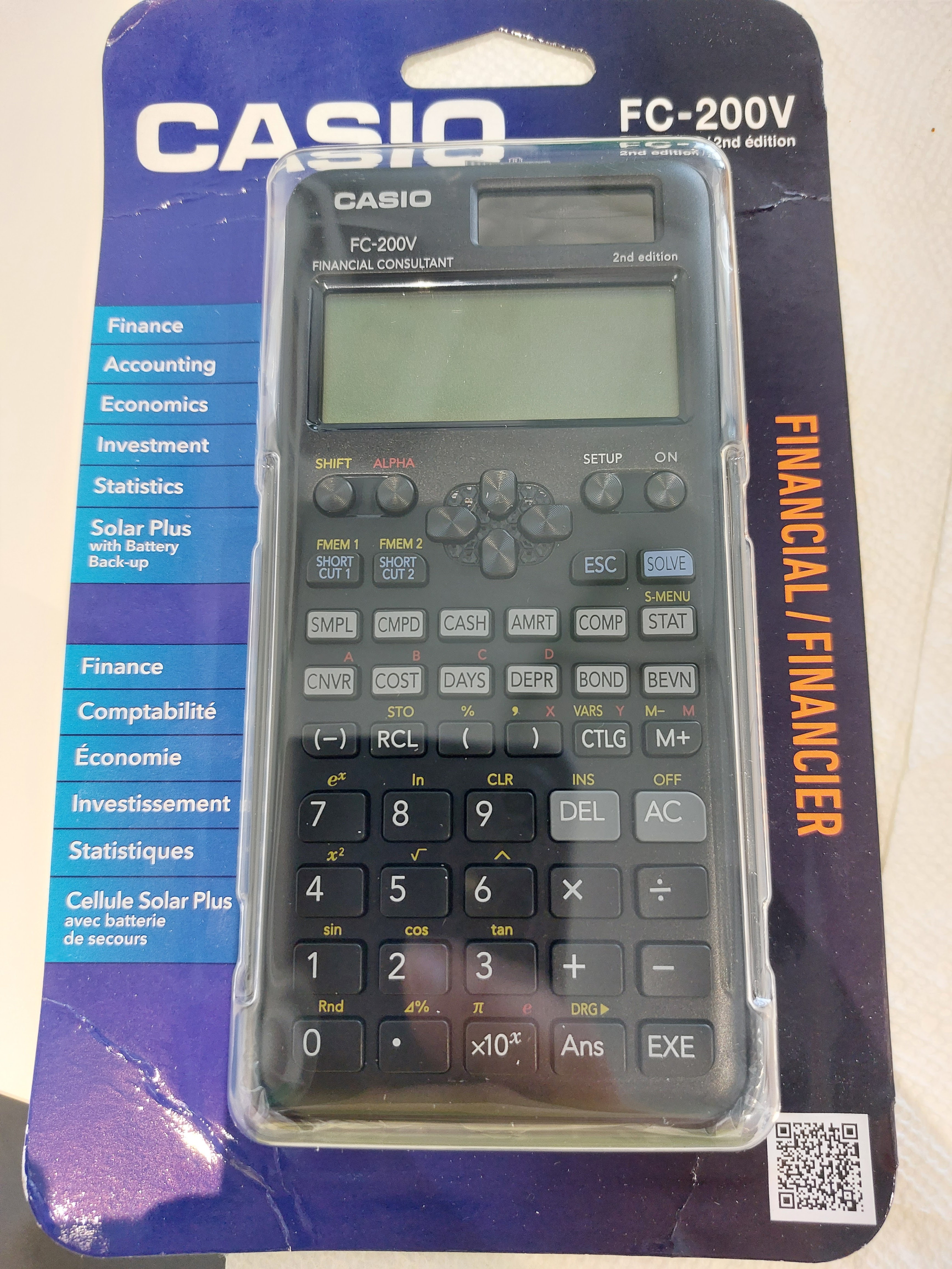
Review: Casio FC-200V 2nd Edition

Review:  Casio FC-200V 2nd Edition

Quick Facts

Model:  FC-200V 2nd Edition

Company:  Casio

Years:  October 2022 - present

Type:  Finance 

Batteries:  Solar and Battery (1 LR44)

Memory: 7 memory registers

System:  Algebraic with Order of Operations

Contrast Setting

The Financial 2nd Edition 

Ten years ago I reviewed the FC-200V "1st edition", which had the gold keyboard.  To be honest, I the cash flow problem I had was probably due to operator error (me).  

The gold 1st edition was released in 2004 and 18 years later, we have the black 2nd edition.  The 2nd edition follows Casio updating the scientific calculators such as fx-115 ES, fx-300 ES, and fx-300 MS.  According to Casio, the redesign are more environmental friendly and more durable than their previous editions.   

Like the fx-115 ES 2nd Edition, the keyboard FC-200V 2nd Edition feels responsive and looks clean.  

The two rows of light gray keys features the worksheets and modes of the FC-200V:

SMPL:  Simple Interest

CPMD:  Compound Interest (Time Value of Money)

CASH:  Cash Flows

AMRT:  Amortization (of compound interest)

COMP:  Compute mode, main mode

STAT:  Statistics

CNVR:  APR/EFF Conversions

COST:  Cost/Sell/Profit Margin Solver

DAYS:  Days Between Dates and Date Calculation

DEPR:  Depreciation

BOND:  Bond Calculations

BEVN:  Breakeven Calculations

The sticker on the case lists all of variables used in the calculator, as well as how to set the contrast on the screen.   

The available regressions are:

A+Bx:  Linear

+Cx^2:  Quadratic

ln X:  Logarithmic

e^X:  Exponential

A∙B^X:  Exponential (any base)

A∙X^B: Power

1/X:  Inverse

We can store up to 80 single data points, or 40 pairs of data points.  Turning STAT mode on in SETUP will give us access to the frequency column.  However this reduces the maximum number of data points to 40 and 26, respectively. 

The types of depreciation models available are:

SL:  Straight Line

FP:  Fixed Percentage

SYD: Sum of the Year's Digits

DB:  Declining Balance

Some of the variables are shared with the time value of money variables:

n = life of the asset

I% = percentage or declining balance factor

PV = cost

FV = residual value or salvage value

The Cash Flow worksheet features the following calculations:

NPV:  net present value

IRR:  internal rate of return

PBP:  payback period

NFV:  net future value 

Be aware that the data entry is shared with the statistics mode.   The first data point is still marked data point 1.  Data point 1 is the initial cash flow, typically labeled CF0 in most calculators.  I wish that the FC-200V had two separate lists in memory for cash flows and statistics to reduce confusion.  Turning STAT mode on in SETUP will allow for each point to have a frequency.   

Switch between statistics and cash flow modes will clear the list of data points.   This is one of the few areas where data does not transfer between applications.  

There is a FC-100V which is battery powered but does not have depreciation, bonds, and breakeven calculations.   The FC-100V 2nd Edition is currently available outside of the United States.  

I think the FC-200V could have used a QR code command on the calculator like the fx-991 EX.  However, we get a QR code on the calculator's case which gives access to the user manual.  

One of my favorite features is the ability to store two expressions through SHORT CUT 1 and SHORT CUT 2, and two functions with the FMEM1 and FMEM2.  FMEM1 and FMEM2 are the only way to assign access some of the functions such as rectangular/polar conversions, arcsine, arccosine, arctangent, factorial, and absolute value to the keyboard.

Variables

The FC-200V has seven variables independent of the financial variables: A, B, C, D, X, Y, and M.  M has the memory add (M+) and memory subtract (M-) that Casio has on scientific calculators.  We can enter variables with the ALPHA key.  However, the store key brings up a menu and this is the only way to store variables.  

The Percent Key and the Percent Change Key

The percent key works like the percent function on scientific algebraic calculators, just dividing its argument by 100.  The percent key (Δ%) also had idiosyncrasies to it.  Just typing Δ% execute the function immediately. 

To add y percent to x:  x + x * y% or x * (1 + y%)

To subtract y percent from x:  x - x * y% or x * (1 - y%)

To calculate percent change from x to y:  x - y Δ%

To calculate (y + x)/x * 100%:  x + y Δ%

To calculate sale price:   cost * profit margin Δ%

The manual makes a great reference, not only detailing the operations of the calculator, but also lists reference formulas.  You will have to find it online, as the calculator only gets quick start guides in English, Spanish, and French.

Final Thoughts

The FC-200V 2nd Edition is a feature rich financial calculator and its pretty easy to use, if you are willing to work with the idiosyncrasies.  

 

  

Source

Casio.  "FC-200V-2 Financial"  Retrieved December 3, 2022.  https://www.casio.com/us/scientific-calculators/product.FC-200V-2/

Eddie

All original content copyright, © 2011-2022.  Edward Shore.   Unauthorized use and/or unauthorized distribution for commercial purposes without express and written permission from the author is strictly prohibited.  This blog entry may be distributed for noncommercial purposes, provided that full credit is given to the author. 

HP Prime: Constant Payment Applied to Principal

HP Prime:  Constant Payment Applied to Principal 

Constant Amount Applied to Principal 

In most loans and mortgages,  the amount of payment applying to interest and principal depends on the running balance.  

This program assumes the customer wants an equal portion to apply to principal each payment.   As a result, the payment itself, principal and interest, will vary.  The simple algorithm to amortize this loan is this:

For K=1 to N:

Int =  Bal * I%÷100

Tpmt = Int + CPMT

Bal_k = Bal_(k-1) - CMPT

where:

Bal = balance of a loan

PV = loan amount

CPMT = amount to be applied to principal each payment

I% = interest rate

Int = interest calculated for payment K

Tpmt = total payment for payment K

HP Prime Program CPYMT

The result of CPYMT is a four column matrix with rows:  k, interest in payment k, total payment k, resulting balance.  Keep in mind that program asks for periodic interest rate.  

EXPORT CPYMT()

BEGIN

// 2022-10-24 EWS

// fix 2

HFormat:=1;

HDigits:=2;

// local

LOCAL n,i,p,b,it,tp,k,x;

LOCAL ll,l0,l1,l2,l3,m;

// main

INPUT({n,i,p,b},"Constant Principal",

{"N = ","I%=","PMT=","LOAN="},

{"# of payments",

"periodic interest rate",

"constant payment",

"loan amount"});

l0:={0};

l1:={0};

l2:={b};

FOR k FROM 1 TO n DO

it:=b*i/100;

tp:=p+it;

b:=b-p;

ll:=MAKELIST(x,x,1,n+1,1);

l0:=CONCAT(l0,{it});

l1:=CONCAT(l1,{tp});

l2:=CONCAT(l2,{b});

END;

l3:=CONCAT(ll,l0);

l3:=CONCAT(l3,l1);

l3:=CONCAT(l3,l2);

m:=list2mat(l3,SIZE(l0));

m:=TRN(m);

RETURN m; 

END;

Example

Five year loan of $10,000 where the customer requests an equal amount of principal to be applied each annual payment ($2,000 a year).  The loan rate is 6.99%.

Inputs:

N = 5

I% = 6.99

PMT = 2,000.00

LOAN = 10,000.00

Result:

Year 1:  Interest:  $699.00;  Total Payment:  $2,699.00;  Balance:  $8,000.00

Year 2:  Interest:  $599.20;  Total Payment:  $2,559.20;  Balance:  $6,000.00

Year 3:  Interest:  $419.40;  Total Payment:  $2,419.40;  Balance:  $4,000.00

Year 4:  Interest:  $279.60;  Total Payment:  $2,279.60;  Balance:  $2,000.00

Year 5:  Interest:  $139.80;  Total Payment:  $2,139.80;  Balance:  $0.00

Source

"Constant Payment to Principal Loan"  HP-41 User's Library Solutions: Lend/Lease/Savings  Hewlett Packard.  November 1980

Next week I am going to cover the legendary HP 75C.  

All original content copyright, © 2011-2022.  Edward Shore.   Unauthorized use and/or unauthorized distribution for commercial purposes without express and written permission from the author is strictly prohibited.  This blog entry may be distributed for noncommercial purposes, provided that full credit is given to the author. 

HP 20S: Triac Waveforms

HP 20S:   Triac Waveforms

Introduction

The following calculations involve triode AC switches, better known as triacs.  A triac is generally used as a bidirectional power switch device.  James J. Davidson, the original author of the HP 25 programs states "these programs are for use with mean-absolute (also called average) responding voltmeters which are calibrated to read the rms value of a sine wave"  (Davidson, 38).

The variables used in Davidson's programs are: 

Vs = root mean square from source

VLMS = root mean square voltage

VLMA = average load voltage

θ = firing angle of triac in degrees (Davidson, 38)

These programs have been translated to for the use of the HP 20S calculator.  

HP 20S Program:  Triac Waveforms

(59 steps)

Given:  Vs and θ°, calculate VLMA and VLMS

Store Vs in R0

Store θ° in R1 (degrees)

Press [ XEQ ] [ A ]

VLMA is displayed

Press [ R/S ], VLMA is displayed

Given:  Vs and VLMA, calculate θ° and VLMS

Store Vs in R0

Store VLMA in R4

Press [ XEQ ] [ B ]

θ° is displayed

Press [ R/S ], VLMA is displayed

Variables:

R0 = Vs

R1 = θ in degrees

R2 = θ in radians

R3 = VLMA 

R4 = VLMS

Program Code

Key Code:  { Key }

61, 41, A:  { LBL A }

61, 24:  { RAD }

22, 1:  { RCL 1 }

61, 55:  { →RAD }

21, 2:  { STO 2 }

24:  { COS }

75:  { + }

1:  { 1 }

74:  { = }

55: { × }

22, 0:  { RCL 0 }

45:  { ÷ }

2:  { 2 }

74:  { = }

21, 3:  { RCL 3 }

26:  { R/S }

51, 41, 1:  { GTO 1 }

61, 26:  { RTN }

61, 41, b:  { LBL B }

61, 24:  { RAD }

33:  { ( }

2:  { 2 }

55:  { × }

22, 3:  { RCL 3 }

45:  { ÷ }

22, 0:  { RCL 0 }

65:  { - }

1:  { 1 }

34:  { ) }

51, 24:  { ACOS }

21, 2:  { STO 2 }

51, 55:  { →DEG }

21, 1:  { STO 1 }

26:  { R/S }

51, 41, 1:  { GTO 1 }

61, 26:  { RTN }

61, 41, 1:  { LBL 1 }

61, 22:  { π }

65:  { - }

22, 2:  { RCL 2 }

75:  { + }

33:  { ( }

2:  { 2 }

55:  { ÷ }

22, 2:  { RCL 2 }

34:  { ) }

23:  { SIN }

45:  { ÷ }

2:  { 2 }

74:  { = }

11:  { √ }

55:  { × }

22, 0:  { RCL 0 }

45:  { ÷ }

61, 22:  { π }

11:  { √ }

74:  { = }

21, 4:  { STO 4 }

61, 26:  { RTN }

Example

Example 1:

Inputs:  θ  = 75° (stored in R1), Vs = 160 (stored in R0)

Results:

VLMA ≈ 100.70552

VLMS ≈ 130.27094

Example 2:

Inputs:  VLMA = 130 (stored in R3), Vs = 160 (stored in R0)

Results:

θ ≈ 51.31781°

VLMS ≈ 149.25534

Source

Davidson, James J.  "Triac Waveforms #1" and "Traic Waveforms #2" 65 Notes V3N10 December 1976.  pg. 38.  

All original content copyright, © 2011-2022.  Edward Shore.   Unauthorized use and/or unauthorized distribution for commercial purposes without express and written permission from the author is strictly prohibited.  This blog entry may be distributed for noncommercial purposes, provided that full credit is given to the author and any authors of original programs and scripts.  

HP 32SII: Random Number Utilities

HP 32SII:  Random Number Utilities

Note:  The following programs should work with the original HP 32S.   The checksums listed are for the HP 32SII only.  

HP 32SII Program:  Fill a Set of Registers with Increasing Integers

This program fills up the alpha registers with consecutive increasing integers.  Up to 25 slots are available, A- Y, with the lowest being stored in A.   Register Z is used to store the difference.  

The difference from both numbers should not be more than 24.  

F01  LBL F

F02  x<>y

F03  1

F04  -

F05 STO Z

F06 -

F07 STO i

I01  LBL I

I02  RCL i

I03  IP

I04  RCL+ Z

I05  STO(i)

I06  DSE i

I07  GTO I

I08  RTN

F:  10.5 bytes, 32SII checksum 9FB9

I:  12.0 bytes, 32SII checksum E189

Total:  22.5 bytes

Examples

18 to 27:   18 ENTER 27 XEQ F

Results:

A = 18, B = 19, C = 20, D = 21, E = 22, 

F = 23, G = 24, H = 25, I = 26, J = 27

HP 32SII Program:  Pick from Registers A through Y

Enter the number of registers to pick from into register Z.  For example, if you have registers A through J loaded, store 10 into register Z.

Note:  When used for indirect addressing, the absolute value of integer of register i is used.   This will allows us to save a few steps.

G01  RANDOM

G02  RCL× Z

G03  1

G04  +

G05  STO i

G06  RCL(i)

G07  RTN

G:  12.0 bytes, 32SII checksum FE18

Example:

Use the data from the last problem.  

10 STO Z, 

XEQ G:   22

XEQ G:   21

(results will vary)

Source for the next two programs:

Chamberlain, Gary.  "HP-29C Random Number Generators"  PPC Journal V6 N7 October 1979

HP 32SII Program:  Uniform Distribution 

This program picks random numbers between two parameters.

U01  LBL U

U02  STO C

U03  -

U04  STO D

W01  LBL W

W02  RANDOM

W03  RCL× D

W04  RCL+ C

W05  STOP

W06  GTO W

U:  6.0  bytes, 32SII checksum 8022

W: 9.0  bytes, 32SII checksum 88EE

Total:  15.0 bytes

Example:

Random numbers between -1 and 1:

XEQ U:  -0.74076 (press R/S for more random numbers)

0.28000

-0.80090

0.20653

0.50614

HP 32SII Program:  Gaussian Distribution of Random Numbers

Generate random numbers that fit on a normal distribution with mean M and deviation D.  Two random numbers are generated, press x<>y to see both results.

X01  LBL X

X02  INPUT M

X03  INPUT D

X04  RAD   (radians mode)

Y01  LBL Y

Y02  RANDOM 

Y03  2 

Y04  ×

Y05  π

Y06  ×

Y07  RANDOM

Y08  LN

Y09  -2

Y10  ×

Y11 SQRT

Y12  θ,r→y,x

Y13  RCL× D

Y14  RCL+ M

Y15  x<>y

Y16  RCL× D

Y17  RCL+ M

Y18  STOP

Y19  GTO Y

Example:

Mean = 3 

Deviation: 1.5

XEQ X

M?  3 R/S

D?  1.5 R/S

1.70434 x<>y 2.89313 R/S

2.22287 x<>y 2.50113 R/S

1.67644 x<>y 2.87034 ...

(results will vary)

Happy programming,

Eddie 

All original content copyright, © 2011-2022.  Edward Shore.   Unauthorized use and/or unauthorized distribution for commercial purposes without express and written permission from the author is strictly prohibited.  This blog entry may be distributed for noncommercial purposes, provided that full credit is given to the author. 

HP 20S: Gamma Function Approximation (Stirling's Formula)

HP 20S:  Gamma Function Approximation (Stirling's Formula)

Introduction

The gamma function uses the approximation sequence:

Let t = x + 9

Then calculate:

Let G = Γ(t) ≈ 

exp( ln √(2 × π ÷ t) + t × ln t - t + (12 × t)^-1 - (360 × t^3)^-1 + (1260 × t^5)^-1 )

Note:

(360 × t^3)^-1  = (12 × t)^-1 × (30 × t^2)^-1

(1260 × t^5)^-1 = (360 × t^3)^-1 × (3.5 × t^2)^-1

While x > t:  

G = G ÷ x

x = x + 1

End Loop

Display G as the final answer 

The approximation polynomial is used for higher values because for the approximation is more accurate for higher values.  

HP 20S:  Gamma Approximation

(63 steps)

Key Code:  { Key }

61, 41, b :  { LBL B }

21, 1 :  { STO 1 }

75 :   { + }

9 :  { 9 }

74 : { = }

21, 2 : { STO 2 }

32 : { +/- }

21, 0 : { STO 0 }

32 : { +/- } 

55 : { × }

13 : { LN }

74 : { = }

21, 75, 0 : { STO+ 0 }

2 :  { 2 }

55 : { × }

61, 22 : { π }

45 : { ÷ }

22, 2 : { RCL 2 }

74 : { = }

11 : { √ }

13 : { LN }

21, 75, 0 : { STO+ 0 }

1 : { 1 }

2 : { 2 }

55 : { × }

22, 2 : { RCL 2 }

74 : { = }

15 : { 1/x }

21, 75, 0 : { STO+ 0 }

45 : { ÷ }

3 : { 3 }

0 : { 0 }

45 : { ÷ }

22, 2 : { RCL 2 }

51, 11 :  { x^2 }

74 : { = }

21, 65, 0 : { STO- 0 }

45 : { ÷ }

3 : { 3 }

73 : { . }

5 : { 5 }

45 : { ÷ }

22, 2 : { RCL 2 }

51, 11 : { x^2 }

74 : { = }

21, 75, 0 : { STO+ 0 }

22, 0 : { RCL 0 }

12 : { e^x }

21, 0 : { STO 0 }

61, 41, 0 : { LBL 0 }

22, 1 : { RCL 1 }

21, 45, 0 : { STO÷ 0 }

1 : { 1 }

21, 75, 1 : { STO+ 1 }

22, 2 : { RCL 2 }

31 : { INPUT }

22, 1 : { RCL 1 }

61, 42 : { x≤y? }

51, 41, 1 : { GTO 1 }

51, 41, 0 : { GTO 0 }

61, 41, 1 : { LBL 1 }

22, 0 : { RCL 0 }

61, 26 : { RTN }

Examples

Γ(0.5) returns 1.77245385109

Γ(4.4) returns 10.1361018514

Calculate the gamma function, press [ XEQ ] B. 

This program is based on the approximation code of the HP 25.  

Source:

Davidson, Jim, and John Vlissides.  "HP-25 Program-Gamma Function"  ENTER: 65 NOTES  Vol. 3 No. 10  December 1976

All original content copyright, © 2011-2022.  Edward Shore.   Unauthorized use and/or unauthorized distribution for commercial purposes without express and written permission from the author is strictly prohibited.  This blog entry may be distributed for noncommercial purposes, provided that full credit is given to the author. 

Casio fx-CG 50: Fresnel's Equations - Polarized Light

Casio fx-CG 50:  Fresnel's Equations - Polarized Light

Introduction:  Reflection and Transmission

The object of Fresnel's Equations is to calculate the reflection and transmissions of a light wave when it hits a change of medium.   Where the change of medium occurs is known as of a plane of incidence.  The equations calculate components:  p-polarized light for light parallel to the plane of incidence, and s-polarized light for perpendicular to the plane of incidence.  

The program presented also calculates Brewster's Angle, the angle required for light to hit the plane of incidence to have no reflection.  

Simplified, the equations are:

Angle of Transmission per Snell's Law:

Θt = arcsin(n1 × sin Θi ÷ n2)

Reflection Coefficients:

r ∥ = tan(Θi - Θt) ÷ tan(Θi + Θt) 

r ⟂ = -sin(Θi - Θt) ÷ sin(Θi + Θt) 

Transmission Coefficients:

t ∥ = (2 × sin Θt × cos Θi) ÷ (sin(Θi + Θt) × cos(Θi - Θt))

t ⟂ = (2 × sin Θt × cos Θi) ÷ sin(Θi + Θt)

Brewster's Angle:

Θb = arctan(Θt ÷ Θi)

Casio fx-CG 50 Program:  POLARIZE

(284 bytes)

Text file:

'ProgramMode:RUN

"2022-10-19 EWS"

Deg

"REFRACT INDEX 1"?->M

"_Theta_I"?->P

"REFRACT INDEX 2"?->N

"_Theta_T"

sin^-1 (M*sin P/N)->QDisps

"REFLECTION:"

"R_#E6D7_:"

tan (P-Q)/tan (P+Q)->RDisps

"R_#E6D5_:"

(-)sin (P-Q)/sin (P+Q)->TDisps

"TRANSMISSION:"

"T_#E6D7_:"

(2*sin Q*cos P)/(sin (P+Q)*cos (P-Q))->SDisps

"T_#E6D5_:"

(2*sin Q*cos P)/sin (P+Q)->UDisps

"BREWSTERS ANGLE:"

tan^-1 (N/M)->B

Program Code:

"2022-10-19 EWS"

Deg

"REFRACT INDEX 1"?→M

"ΘI"?→P

"REFRACT INDEX 2"?→N

"ΘT"

sin^-1 (M*sin P/N)→Q ◢

"REFLECTION:"

"R∥:"

tan (P-Q)/tan (P+Q)→R ◢

"R⟂:"

-sin (P-Q)/sin (P+Q)→T ◢

"TRANSMISSION:"

"T∥:"

(2*sin Q*cos P)/(sin (P+Q)*cos (P-Q))→S ◢

"T⟂:"

(2*sin Q*cos P)/sin (P+Q)→U ◢

"BREWSTERS ANGLE:"

tan^-1 (N/M)→B

The symbols ∥ and ⟂ are from the CHAR menu.  

Examples

All angles are in degrees.  

Example 1:

Inputs:

n1 = 1.00293 

ΘI = 20

n2 = 1.52 (glass)

Results:

ΘT = 13.04242914

R∥ = 0.1876099408

R⟂ = -0.2221588123

T∥ = 0.7836116039

T⟂ = 0.7778411877

Brewster's Angle = 56.58227879

Example 2:

Inputs:

n1 = 1.000293 (air)

ΘI = 34

n2 = 1.333 (water)

Results:

ΘT = 24.81075448

R∥ = 0.09793113211

R⟂ = -0.1866780705

T∥ = 0.8238955934

T⟂ = 0.8133219295

Brewster's Angle = 53.11516797

Sources

"Brewster's Angle".  Wikipedia.  https://en.wikipedia.org/wiki/Brewster%27s_angle  Retrieved October 18, 2022

"Fresnel's Equations: Reflection and Transmission"  HyperPhysics. http://hyperphysics.phy-astr.gsu.edu/hbase/phyopt/freseq.html  Retrieved October 16, 2022

Until next time,

Eddie

All original content copyright, © 2011-2022.  Edward Shore.   Unauthorized use and/or unauthorized distribution for commercial purposes without express and written permission from the author is strictly prohibited.  This blog entry may be distributed for noncommercial purposes, provided that full credit is given to the author. 

HP 15C and TI-84 Plus CE: Weibull Distribution Parameter Calculation

HP 15C and TI-84 Plus CE:  Weibull Distribution Parameter Calculation

Introduction

The Weibull probability density distribution function is:

f(x) = (b / Θ) * (x / Θ)^(b-1) * exp(-(x / Θ)^b)

with the lower tail cumulative distribution of (-∞ to x):

Area = 1 - exp(-(x / Θ)^b)

The area function tells us what is the probability a device lasts no more than x time units.  

Area = 1 - Survival

The survival function is the probability a device lasts more than x time units.

Survival = exp(-(x / Θ)^b)

Generally, the higher Θ is, the flatter the Weibull Distribution curve.  

In today's blog, we are estimating the parameters b and Θ given the number of data points, N, and data points (time periods to failure) x_i.   For the HP 15C program, which is modeled after the HP 55 program (see source below).   

The Process

Each x_i is sorted in ascending order.  Then transform the following data:

x' = ln x

α = (K - 0.3) ÷ (N + 0.4),  K = 1, 2, 3, ... , N

y' = ln( ln( 1 ÷ (1 - α)))

Enter each point (x', y'), and perform a linear regression analysis.

Then:  

b = slope

Θ = e^-(intercept ÷ slope)

 

HP 15C Program:  Weibull Distribution - Parameter Determination

Line #;  Key;  Code

001;  LBL A; 42, 21, 11

002;  1;  1

003;  STO 0;  44, 0

004;  CLΣ;  43, 32

005;  R/S;  31

006;  STO 1;  44, 1

007;  LBL 9;  42, 21, 9

008;  R/S;   31

009;  LN;  43, 12

010;  RCL 0;  45, 0

011;  . ;  48

012;  3 ;  3

013;  - ;  30

014; RCL 1;  45, 1

015; .  ;  48

016; 4 ;  4

017; +  ; 40

018; ÷ ; 10

019; 1 ;  1

020;  STO+ 0;  44, 40, 0

021;  x<>y  ; 34

022;  - ; 30

023;  1/x ;  15

024;  LN ; 43, 12

025;  LN ; 43, 12

026;  x<>y ; 34

027;  Σ+ ; 49

028;  GTO 9; 22, 9

029;  LBL B; 42, 21, 12

030;  L.R.;  42, 49

031;  x<>y ; 34

032;  R/S ; 31

033;  ÷ ; 10

034;  CHS;  16

035;  e^x;  12

036;  RTN;  43, 32

1.  Execute label A.   

2.  Enter N, the number of data points, then press the R/S key.

3.  Enter each x_i in ascending order, press R/S key in between each keys.  

4.  Execute label B.   The b parameter is displayed.  

5.  Press R/S.  The Θ parameter is displayed.

TI-84 Plus CE Program: WBFIT  

Weibull Distribution - Parameter Determination

"EWS 2022-10-09"

ClrHome

Disp "WEIBULL DIST.","FIT CALCULATION"

Input "DATA LIST: ",L1

SortA(L1)

dim(L1)→N

ln(L1)→L1

N→dim(L2)

For(K,1,N)

(K-0.3)/(N+0.4)→A

ln(ln(1/(1-A)))→L2(K)

End

LinReg(a+bx) L1,L2

b→B

e^(­(a/b))→θ

ClrHome

Disp "1-e^(­(X/B)^θ)"

Disp "B:",B,"θ:",θ

The x_i data are sorted in the WBIT program.  

Examples

Example 1:

Hours to failure:

{ 11000, 11056, 11379, 11821, 11956, 12403, 12526, 13000, 13380, 13663 }

N = 10

b ≈ 14.01123

Θ ≈ 12649.59071

Example 2:

Days to failure:

{ 1760, 1799, 1882, 1931, 1996, 2004, 2150 }

N = 7

b ≈ 15.22473

Θ ≈ 1993.22461

Sources:

HP55 Statistics Programs  Hewlett Packard Company.  Cupertino, CA.  1975

Ma, Dan.  "The Weibull distribution"  Topics in Actuarial Modeling.  September 28, 2016.   https://actuarialmodelingtopics.wordpress.com/2016/09/28/the-weibull-distribution/  Last Retrieved September 20, 2022.  

Eddie

All original content copyright, © 2011-2022.  Edward Shore.   Unauthorized use and/or unauthorized distribution for commercial purposes without express and written permission from the author is strictly prohibited.  This blog entry may be distributed for noncommercial purposes, provided that full credit is given to the author.